8 The R package `wrassp`¹⁵

8.1 Introduction

This chapter gives an overview and introduction to the wrassp package. The wrassp package is a wrapper for R around Michel Scheffers’ libassp (Advanced Speech Signal Processor). The libassp library and therefore the wrassp package provide functionality for handling speech signal files in most common audio formats and for performing signal analyses common in the phonetic and speech sciences. As such, wrassp fills a gap in the R package landscape as, to our knowledge, no previous packages provided this specialized functionality. The currently available signal processing functions provided by wrassp are:

acfana(): Analysis of short-term autocorrelation function
afdiff(): Computes the first difference of the signal
affilter(): Filters the audio signal (e.g., low-pass and high-pass)
cepstrum(): Short-term cepstral analysis
cssSpectrum(): Cepstral smoothed version of dftSpectrum()
dftSpectrum(): Short-term DFT spectral analysis
forest(): Formant estimation
ksvF0(): F0 analysis of the signal
lpsSpectrum(): Linear predictive smoothed version of dftSpectrum()
mhsF0(): Pitch analysis of the speech signal using Michel Scheffers’ Modified Harmonic Sieve algorithm
rfcana(): Linear prediction analysis
rmsana(): Analysis of short-term Root Mean Square amplitude
zcrana(): Analysis of the averages of the short-term positive and negative zero-crossing rates

The available file handling functions are:

read.AsspDataObj(): read a SSFF or audio file into an AsspDataObj, which is the in-memory equivalent of the SSFF or audio file.
write.AsspDataObj(): write an AsspDataObj to file (usually SSFF or audio file formats).

See R’s help() function for a comprehensive list of every function and object provided by the wrassp package is required (see R code snippet below).

help(package="wrassp")

As the wrassp package can be used independently of the EMU-SDMS this chapter largely focuses on using it as an independent component. However, Section 8.7 provides an overview of how the package is integrated into the EMU-SDMS. Further, although the wrassp package has its own set of example audio files (which can be accessed in the directory provided by system.file('extdata', package='wrassp')), this chapter will use the audio and SSFF files that are part of the ae emuDB of the demo data provided by the emuR package. This is done primarily to provide an overview of what it is like using wrassp to work on files in an emuDB. The R code snippet below shows how to generate this demo data followed by a listing of the files contained in a directory of a single bundle called msajc003 (see Chapter 5 for information about the emuDB format). The output of the call to list.files() shows four files where the .dft and .fms files are in the SSFF file format (see Appendix 15.1.3 for further details). The _annot.json file contains the annotation information, and the .wav file is one of the audio files that will be used in various signal processing examples in this chapter.

# load the emuR package
library(emuR)

# create demo data in directory
# provided by tempdir()
create_emuRdemoData(dir = tempdir())

# create path to demo database
path2ae = file.path(tempdir(), "emuR_demoData", "ae_emuDB")

# load database
# (verbose = F is only set to avoid additional output in manual)
ae = load_emuDB(path2ae, verbose = F)

# create path to bundle in database
path2bndl = file.path(path2ae, "0000_ses", "msajc003_bndl")

# list files in bundle directory
list.files(path2bndl)

## [1] "msajc003_annot.json" "msajc003.dft"        "msajc003.fms"       
## [4] "msajc003.wav"

8.2 File I/0 and the `AsspDataObj`

One of the aims of wrassp is to provide mechanisms for handling speech-related files such as audio files and derived and complementary signal files. To have an in-memory object that can hold these file types in a uniform way the wrassp package provides the AsspDataObj data type. The R code snippet below shows how the read.AsspDataObj() can be used to import a .wav audio file into R.

# load the wrassp package
library(wrassp)

## Loading required package: tibble

# create path to wav file
path2wav = file.path(path2bndl, "msajc003.wav")

# read audio file
au = read.AsspDataObj(path2wav)

# show class
class(au)

## [1] "AsspDataObj"

# show print() output of object
au

## Assp Data Object of file /tmp/RtmpObIFse/emuR_demoData/ae_emuDB/0000_ses/msajc003_bndl/msajc003.wav.
## Format: WAVE (binary)
## 58089 records at 20000 Hz
## Duration: 2.904450 s
## Number of tracks: 1 
##   audio (1 fields)

As can be seen in the above R code snippet, the resulting au object is of the class AsspDataObj. The output of print provides additional information about the object, such as its sampling rate, duration, data type and data structure information. Since the file we loaded is audio only, the object contains exactly one track. Further, since it is a mono file, this track only has a single field. We will later encounter different types of data with more than one track and multiple fields per track. The R code snippet below shows function calls that extract the various attributes from the object (e.g., duration, sampling rate and the number of records).

# show duration
dur.AsspDataObj(au)

## [1] 2.90445

# show sampling rate
rate.AsspDataObj(au)

## [1] 20000

# show number of records/samples
numRecs.AsspDataObj(au)

## [1] 58089

# show additional attributes
attributes(au)

## $names
## [1] "audio"
## 
## $trackFormats
## [1] "INT16"
## 
## $sampleRate
## [1] 20000
## 
## $filePath
## [1] "/tmp/RtmpObIFse/emuR_demoData/ae_emuDB/0000_ses/msajc003_bndl/msajc003.wav"
## 
## $origFreq
## [1] 0
## 
## $startTime
## [1] 0
## 
## $startRecord
## [1] 1
## 
## $endRecord
## [1] 58089
## 
## $class
## [1] "AsspDataObj"
## 
## $fileInfo
## [1] 21  2

The sample values belonging to a trackdata objects tracks are also stored within an AsspDataObj object. As mentioned above, the currently loaded object contains a single mono audio track. Accessing the data belonging to this track, in the form of a matrix, can be achieved using the track’s name in combination with the $ notation known from R’s common named list object. Each matrix has the same number of rows as the track has records and as many columns as the track has fields. The R code snippet below shows how the audio track can be accessed.

# show track names
tracks.AsspDataObj(au)

## [1] "audio"

# or an alternative way to show track names
names(au)

## [1] "audio"

# show dimensions of audio attribute
dim(au$audio)

## [1] 58089     1

# show first sample value of audio attribute
head(au$audio, n = 1)

##      [,1]
## [1,]   64

This data can, for example, be used to generate an oscillogram of the audio file as shown in the R code snippet below, which produces Figure 8.1.

# calculate sample time of every 10th sample
samplesIdx = seq(0, numRecs.AsspDataObj(au) - 1, 10)
samplesTime = samplesIdx / rate.AsspDataObj(au)

# extract every 10th sample using window() function
samples = window(au$audio, deltat=10)

# plot samples stored in audio attribute
# (only plot every 10th sample to accelerate plotting)
plot(samplesTime,
     samples,
     type = "l",
     xlab = "time (s)",
     ylab = "Audio samples (INT16)")

Figure 8.1: Oscillogram generated from samples stored in the audio track of the object au.

The export counterpart to read.AsspDataObj() function is write.AsspDataObj(). It is used to store in-memory AsspDataObj objects to disk and is particularly useful for converting other formats to or storing data in the SSFF file format as described in Section 8.8. To show how this function can be used to write a slightly altered version of the au object to a file, the R code snippet below initially multiplies all the sample values of au$audio by a factor of 0.5. The resulting AsspDataObj is then written to an audio file in a temporary directory provided by R’s tempdir() function.

# manipulate the audio samples
au$audio = au$audio * 0.5
# write to file in directory
# provided by tempdir()
write.AsspDataObj(au, file.path(tempdir(), 'newau.wav'))

8.3 Signal processing

As mentioned in the introduction to this chapter, the wrassp package is capable of more than just the mere importing and exporting of specific signal file formats. This section will focus on demonstrating three of wrassp’s signal processing functions that calculate formant values, their corresponding bandwidths, the fundamental frequency contour and the RMS energy contour. Section 8.5 and 8.5.1 demonstrates signal processing to the audio file saved under path2wav, while Section 8.5.2 adresses processing all the audio files belonging to the ae emuDB.

8.4 The `wrasspOutputInfos` object

The wrassp package comes with the wrasspOutputInfos object, which provides information about the various signal processing functions provided by the package. The wrasspOutputInfos object stores meta information associated with the different signal processing functions wrassp provides. The R code snippet below shows the names of the wrasspOutputInfos object which correspond to the function names listed in the introduction of this chapter.

# show all function names
names(wrasspOutputInfos)

##  [1] "acfana"      "afdiff"      "affilter"    "cepstrum"    "cssSpectrum"
##  [6] "dftSpectrum" "ksvF0"       "mhsF0"       "forest"      "lpsSpectrum"
## [11] "rfcana"      "rmsana"      "zcrana"

This object can be useful to get additional information about a specific wrassp function. It contains information about the default file extension ($ext), the tracks produced ($tracks) and the output file type ($outputType). The R code snippet below shows this information for the forest() function.

# show output info of forest function
wrasspOutputInfos$forest

## $ext
## [1] "fms"
## 
## $tracks
## [1] "fm" "bw"
## 
## $outputType
## [1] "SSFF"

The examples that follow will make use of this wrasspOutputInfos object mainly to acquire the default file extensions given by a specific wrassp signal processing function.

8.5 Formants and their bandwidths

The already mentioned forest() is wrassp’s formant estimation function. The default behavior of this formant tracker is to calculate the first four formants and their bandwidths. The R code snippet below shows the usage of this function. As the default behavior of every signal processing function provided by wrassp is to store its result to a file, the toFile parameter of forest() is set to FALSE to prevent this behavior. This results in the same AsspDataObj object as when exporting the result to file and then importing the file into R using read.AsspDataObj(), but circumvents the disk reading/writing overhead.

# calculate formants and corresponding bandwidth values
fmBwVals = forest(path2wav, toFile = F)

# show class vector
class(fmBwVals)

## [1] "AsspDataObj"

# show track names
tracks.AsspDataObj(fmBwVals)

## [1] "fm" "bw"

# show dimensions of "fm" track
dim(fmBwVals$fm)

## [1] 581   4

# check dimensions of tracks are the same
all(dim(fmBwVals$fm) == dim(fmBwVals$bw))

## [1] TRUE

As can be seen in the above R code snippet, the object resulting from the forest() function is an object of class AsspDataObj with the tracks "fm" (formants) and "bw" (formant bandwidths), where both track matrices have four columns (corresponding to F1, F2, F3 and F4 in the "fm" track and F1_bandwidth, F2_bandwidth, F3_bandwidth and F4_bandwidth in the "bw" track) and 581 rows. To visualize the calculated formant values, the R code snippet below shows how R’s matplot() function can be used to produce Figure 8.2.

# plot the formant values
matplot(seq(0, numRecs.AsspDataObj(fmBwVals) - 1)
        / rate.AsspDataObj(fmBwVals)
        + attr(fmBwVals, "startTime"),
        fmBwVals$fm,
        type = "l",
        xlab = "time (s)",
        ylab = "Formant frequency (Hz)")
# add legend
startFormant = 1
endFormant = 4
legend("topright",
       legend = paste0("F", startFormant:endFormant),
       col = startFormant:endFormant,
       lty = startFormant:endFormant,
       bg = "white")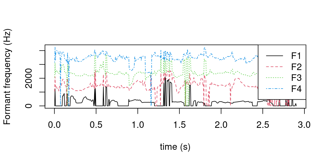

Figure 8.2: Matrix plot of formant values stored in the fm track of fmBwVals object.

8.5.1 Fundamental frequency contour

The wrassp package includes two fundamental frequency estimation functions called ksvF0() and mhsF0(). The R code snippet below shows the usage of the ksvF0() function, this time not utilizing the toFile parameter but rather to show an alternative procedure, reading the resulting SSFF file produced by it. It is worth noting that every signal processing function provided by wrassp creates a result file in the same directory as the audio file it was processing (except if the outputDirectory parameter is set otherwise). The default extension given by the ksvF0() is stored in wrasspOutputInfos$ksvF0$ext, which is used in the R code snippet below to create the newly generated file’s path.

# calculate the fundamental frequency contour
ksvF0(path2wav)

# create path to newly generated file
path2f0file = file.path(path2bndl,
                    paste0("msajc003.",
                           wrasspOutputInfos$ksvF0$ext))

# read file from disk
f0vals = read.AsspDataObj(path2f0file)

Analogous to the formant estimation example, the R code snippet below shows how the plot() function can be used to visualize this data as in Figure 8.3.

# plot the fundamental frequency contour
plot(seq(0,numRecs.AsspDataObj(f0vals) - 1)
     / rate.AsspDataObj(f0vals) +
       attr(f0vals, "startTime"),
     f0vals$F0,
     type = "l",
     xlab = "time (s)",
     ylab = "F0 frequency (Hz)")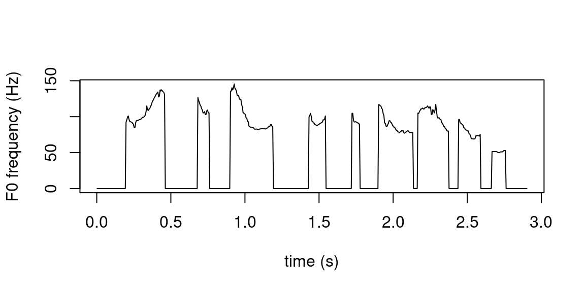

Figure 8.3: Plot of fundamental frequency values stored in the F0 track of f0vals object.

8.5.2 RMS energy contour

The wrassp function for calculating the short-term root mean square (RMS) amplitude of the signal is called rmsana(). As its usage is analogous to the above examples, here we will focus on using it to calculate the RMS values for all the audio files of the ae emuDB. The R code snippet below initially uses the list_files() function to aquire the file paths for every .wav file in the ae emuDB. As every signal processing function accepts one or multiple file paths, these file paths can simply be passed in as the main argument to the rmsana() function. As all of wrassp’s signal processing functions place their generated files in the same directory as the audio file they process, the rmsana() function will automatically place every .rms into the correct bundle directory.

# list all .wav files in the ae emuDB
paths2wavFiles = list_files(ae, fileExtension = "wav")$absolute_file_path

# calculate the RMS energy values for all .wav files
rmsana(paths2wavFiles)

# list new .rms files using
# wrasspOutputInfos->rmsana->ext
rmsFPs = list.files(path2ae,
                    pattern = paste0(".*",
                                     wrasspOutputInfos$rmsana$ext),
                    recursive = TRUE,
                    full.names = TRUE)

# read first RMS file
rmsvals = read.AsspDataObj(rmsFPs[1])

The R code snippet below shows how the plot() function can be used to visualize this data as in Figure 8.4.

# plot the RMS energy contour
plot(seq(0, numRecs.AsspDataObj(rmsvals) - 1)
     / rate.AsspDataObj(rmsvals)
     + attr(rmsvals, "startTime"),
     rmsvals$rms,
     type = "l",
     xlab = "time (s)",
     ylab = "RMS energy (dB)")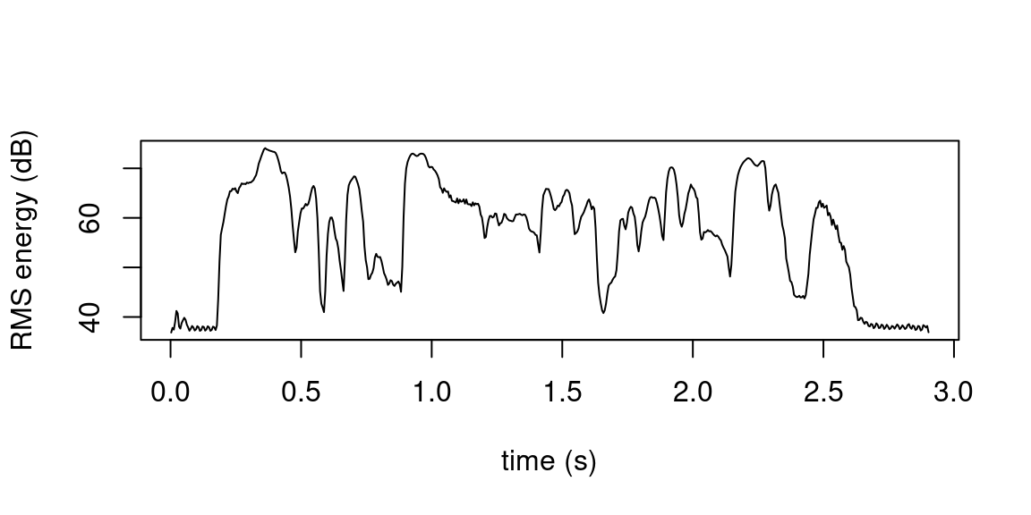

Figure 8.4: Plot of RMS values stored in rms track of the rmsvals object.

8.6 Logging `wrassp`’s function calls

As it can be extremely important to keep track of information about how certain files are created and calculated, every signal processing function provided by the wrassp package comes with the ability to log its function calls to a specified log file. The R code snippet below shows a call to the ksvF0() function where a single parameter was changed from its default value (windowShift = 10). The content of the created log files (shown by the call to readLines()) contains the function name, time stamp, parameters that were altered and processed file path information. It is worth noting that a log file can be reused for multiple function calls as the log function does not overwrite an existing file but merely appends new log information to it.

# create path to log file in root dir of ae emuDB
path2logFile = file.path(path2ae, "wrassp.log")

# calculate the fundamental frequency contour
ksvF0(path2wav, 
      windowShift = 10,
      forceToLog = T, 
      optLogFilePath = path2logFile)

## [1] 1

# display content of log file (first 8 lines)
readLines(path2logFile)[1:8]

## [1] ""                                   "##################################"
## [3] "##################################" "######## ksvF0 performed ########" 
## [5] "Timestamp:  2021-02-15 17:14:05 "   "windowShift : 10 "                 
## [7] "forceToLog : T "                    " => on files:"

8.7 Using `wrassp` in the EMU-SDMS

As shown in Section 8.5.2, the wrassp signal processing functions can be used to calculate SSFF files and place them into the appropriate bundle directories. The only thing that has to be done to make an emuDB aware of these files is to add an SSFF track definition to the emuDB as shown in the R code snippet below. Once added, this SSFF track can be referenced via the ssffTrackName parameter of the get_trackdata() function as shown in various examples throughout this documentation. It is worth noting that this strategy is not necessarily relevant for applying the same signal processing to an entire emuDB, as this can be achieved using the on-the-fly add_ssffTrackDefinition() method described in the according R code snippet below. However, it becomes necessary if certain bundles are to be processed using deviating function parameters. This can, for example, be relevant when setting the minimum and maximum frequencies that are to be considered while estimating the fundamental frequencies (e.g., the maxF and minF of ksvfF0()) for female versus male speakers.

# load emuDB
ae = load_emuDB(path2ae)

# add SSFF track defintion
# that references the .rms files
# calculated above
# (i.e. no new files are calculated and added to the emuDB)
ext = wrasspOutputInfos$rmsana$ext
colName = wrasspOutputInfos$rmsana$tracks[1]
add_ssffTrackDefinition(ae,
                        name = "rms",
                        fileExtension = ext,
                        columnName = colName)

A further way to utilize wrassp’s signal processing functions as part of the EMU-SDMS is via the onTheFlyFunctionName and onTheFlyParams parameters of the add_ssffTrackDefinition() and get_trackdata() functions. Using the onTheFlyFunctionName parameter in the add_ssffTrackDefinition() function automatically calculates the SSFF files while also adding the SSFF track definition. Using this parameter with the get_trackdata() function calls the given wrassp function with the toFile parameter set to FALSE and extracts the matching segments and places them in the resulting trackdata or emuRtrackdata object. In many cases, this avoids the necessity of having SSFF track definitions in the emuDB. In both functions, the optional onTheFlyParams parameter can be used to specify the parameters that are passed into the signal processing function. The R code snippet below shows how R’s formals() function can be used to get all the parameters of wrassp’s short-term positive and negative zero-crossing rate (ZCR) analysis function zrcana(). It then changes the default window size parameter to a new value and passes the parameters object into the add_ssffTrackDefinition() and get_trackdata() functions.

# get all parameters of zcrana
zcranaParams = formals("zcrana")

# show names of parameters
names(zcranaParams)

##  [1] "listOfFiles"     "optLogFilePath"  "beginTime"       "centerTime"     
##  [5] "endTime"         "windowShift"     "windowSize"      "toFile"         
##  [9] "explicitExt"     "outputDirectory" "forceToLog"      "verbose"

# change window size from the default
# value of 25 ms to 50 ms
zcranaParams$windowSize = 50

# to have a segment list to work with
# query all Phonetic 'n' segments
sl = query(ae, "Phonetic == n")

# get trackdata calculating ZCR values on-the-fly
# using the above parameters. Note that no files
# are generated.
# (verbose = F is only set to avoid additional output in manual)
td = get_trackdata(ae, sl,
                   onTheFlyFunctionName = "zcrana",
                   onTheFlyParams = zcranaParams,
                   verbose = FALSE)


# add SSFF track definition. Note that
# this time files are generated.
# (verbose = F is only set to avoid additional output in manual)
add_ssffTrackDefinition(ae,
                        name = "zcr",
                        onTheFlyFunctionName = "zcrana",
                        onTheFlyParams = zcranaParams,
                        verbose = FALSE)

8.8 Storing data in the SSFF file format

One of the benefits gained by having the AsspDataObj in-memory object is that these objects can be constructed from scratch in R, as they are basically simple list objects. This means, for example, that any set of n-dimensional samples over time can be placed in a AsspDataObj and then stored as an SSFF file using the write.AsspDataObj() function. To show how this can be done, the R code snippet below creates an arbitrary data sample in the form of a single cycle sine wave between $0$ and $2*pi$ that is made up of 16000 samples and displays it in Figure 8.5.

x = seq(0, 2 * pi, length.out = 16000)
sineWave = sin(x)
plot(x, sineWave, type = 'l',
     xlab = "x from 0 to 2*pi",
     ylab = "")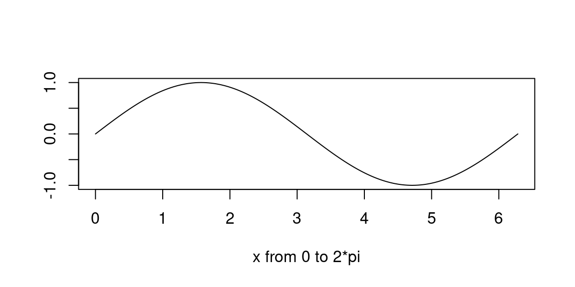

Figure 8.5: A single cycle sine wave consisting of 16000 samples.

Assuming a sample rate of 16 kHz sineWave would result in a sine wave with a frequency of 1 Hz and a duration of one second. The R code snippet below shows how a AsspDataObj can be created from scratch and the data in sineWave placed into one of its tracks. It then goes on to write the AsspDataObj object to an SSFF file.

# create empty list object
ado = list()

# add sample rate attribute
attr(ado, "sampleRate") = 16000

# add start time attribute
attr(ado, "startTime") = 0

# add start record attribute
attr(ado, "startRecord") = as.integer(1)

# add end record attribute
attr(ado, "endRecord") = as.integer(length(sineWave))

# set class of ado
class(ado) = "AsspDataObj"

# show available file formats
AsspFileFormats

##     RAW   ASP_A   ASP_B   XASSP  IPDS_M  IPDS_S    AIFF    AIFC     CSL    CSRE 
##       1       2       3       4       5       6       7       8       9      10 
##    ESPS     ILS     KTH   SWELL   SNACK     SFS     SND      AU    NIST  SPHERE 
##      11      12      13      13      13      14      15      15      16      16 
## PRAAT_S PRAAT_L PRAAT_B    SSFF    WAVE  WAVE_X  XLABEL    YORK     UWM 
##      17      18      19      20      21      22      24      25      26

# set file format to SSFF
# NOTE: assignment of "SSFF" also possible
AsspFileFormat(ado) = as.integer(20)

# set data format (1 == 'ascii' and 2 == 'binary')
AsspDataFormat(ado) = as.integer(2)

# set track format specifiers
# (available track formats for numbers
# that match their C equivalent are:
# "UINT8"; "INT8"; "UINT16"; "INT16";
# "UINT24"; "INT24"; "UINT32"; "INT32";
# "UINT64"; "INT64"; "REAL32"; "REAL64");
attr(ado, "trackFormats") = c("REAL32")

# add track
ado = addTrack(ado, "sine", sineWave, "REAL32")

# write AsspDataObj object to file
write.AsspDataObj(dobj = ado,
                  file = file.path(tempdir(), "example.sine"))

## NULL

Although somewhat of a generic example, the above R code snippet shows how to generate an AsspDataObj from scratch. This approach can, for example, be used to read in signal data produced by other software or signal data acquisition devices. Hence, this approach can be used to import many forms of data into the EMU-SDMS. Appendix 19.1 shows an example of how this approach can be used to take advantage of Praat’s signal processing capabilities and integrate its output into the EMU-SDMS.

8.9 Conclusion

The wrassp packages enriches the R package landscape by providing functionality for handling speech signal files in most common audio formats and for performing signal analyses common in the phonetic and speech sciences. The EMU-SDMS utilizes the functionality that the wrassp package provides by allowing the user to calculate signals that match the segments of a segment list. This can either be done in real time or by extracting the signals from files. Hence, the wrassp package is an integral part of the EMU-SDMS but can also be used as a standalone package if so desired.

Some examples of this chapter are adapted version of examples given in the legacy wrassp_intro vignette of the wrassp package.↩︎

8 The R package wrassp15