7 Signal data extraction14
As mentioned in the default workflow of Chapter 2, after querying the symbolic annotation structure and dereferencing its time information, the result is a set of items with associated time stamps. It was necessary that the emuR package contain a mechanism for extracting signal data corresponding to this set of items. As illustrated in Chapter 8, wrassp provides the R ecosystem with signal data file handling capabilities as well as numerous signal processing routines. emuR can use this functionality to either obtain pre-stored signal data or calculate derived signal data that correspond to the result of a query. Figure 7.1A shows a snippet of speech with overlaid annotations where the resulting SEGMENT of an example query (e.g., "Phonetic == ai") is highlighted in yellow. Figure 7.1B displays a time parallel derived signal data contour as would be returned by one of wrassp’s file handling or signal processing routines. The yellow segment in Figure 7.1B marks the corresponding samples that belong to the ai segment of Figure 7.1A.
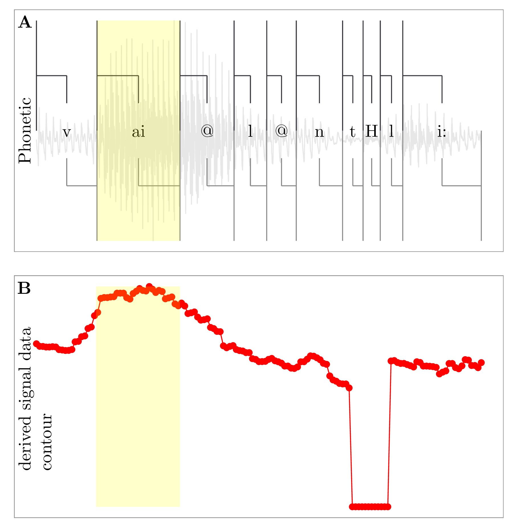
Figure 7.1: Segment of speech with overlaid annotations and time parallel derived signal data contour.
The R code snippet below shows how to create the demo data that will be used throughout this chapter.
# load the package
library(emuR)

# create demo data in directory provided by the tempdir() function
create_emuRdemoData(dir = tempdir())

# get the path to a emuDB called "ae" that is part of the demo data
path2directory = file.path(tempdir(),
                           "emuR_demoData",
                           "ae_emuDB")

# load emuDB into current R session
ae = load_emuDB(path2directory)
7.1 Extracting pre-defined tracks
To access data that are stored in files, the user has to define tracks for a database that point to sequences of samples in files that match a user-specified file extension. The user-defined name of such a track can then be used to reference the track in the signal data extraction process. Internally, emuR uses wrassp to read the appropriate files from disk, extract the sample sequences that match the result of a query and return values to the user for further inspection and evaluation. The R code snippet below shows how a signal track that is already defined in the ae demo database can be extracted for all annotation items on the Phonetic level containing the label ai.
# list currently available tracks
list_ssffTrackDefinitions(ae)
## name columnName fileExtension
## 1 dft dft dft
## 2 fm fm fms# query all "ai" phonetic segments
ai_segs = query(ae, "Phonetic == ai")
# get "fm" track data for these segments
# (verbose = F is only set to avoid additional output in manual)
ai_td_fm = get_trackdata(ae,
seglist = ai_segs,
ssffTrackName = "fm",
verbose = FALSE)
# show ai_td_fm (F1-F4 in columns T1-T4)
ai_td_fm## # A tibble: 183 x 24
## sl_rowIdx labels start end db_uuid session bundle start_item_id end_item_id
## <int> <chr> <dbl> <dbl> <chr> <chr> <chr> <int> <int>
## 1 1 ai 863. 1016. 0fc618… 0000 msajc… 161 161
## 2 1 ai 863. 1016. 0fc618… 0000 msajc… 161 161
## 3 1 ai 863. 1016. 0fc618… 0000 msajc… 161 161
## 4 1 ai 863. 1016. 0fc618… 0000 msajc… 161 161
## 5 1 ai 863. 1016. 0fc618… 0000 msajc… 161 161
## 6 1 ai 863. 1016. 0fc618… 0000 msajc… 161 161
## 7 1 ai 863. 1016. 0fc618… 0000 msajc… 161 161
## 8 1 ai 863. 1016. 0fc618… 0000 msajc… 161 161
## 9 1 ai 863. 1016. 0fc618… 0000 msajc… 161 161
## 10 1 ai 863. 1016. 0fc618… 0000 msajc… 161 161
## # … with 173 more rows, and 15 more variables: level <chr>, attribute <chr>,
## # start_item_seq_idx <int>, end_item_seq_idx <int>, type <chr>,
## # sample_start <int>, sample_end <int>, sample_rate <int>, times_orig <dbl>,
## # times_rel <dbl>, times_norm <dbl>, T1 <int>, T2 <int>, T3 <int>, T4 <int>Being able to access data that is stored in files is important for two main reasons. Firstly, it is possible to generate files using external programs such as VoiceSauce (Shue et al. 2011), which can export its calculated output to the general purpose SSFF file format. This file mechanism is also used to access data produced by EMA, EPG or many other forms of signal data recordings. Secondly, it is possible to track, save and access manipulated data such as formant values that have been manually corrected. It is also worth noting that the get_trackdata() function has a predefined track which is always available without it having to be defined. The name of this track is MEDIAFILE_SAMPLES which references the actual samples of the audio files of the database. The R code snippet below shows how this predefined track can be used to access the audio samples belonging to the segments in ai_segs.
# get media file samples
# (verbose = F is only set to avoid additional output in manual)
ai_td_mfs = get_trackdata(ae,
                          seglist = ai_segs,
                          ssffTrackName = "MEDIAFILE_SAMPLES",
                          verbose = FALSE)

# ai_td_mfs (sample values in column T1)
ai_td_mfs
## # A tibble: 18,386 x 21
## sl_rowIdx labels start end db_uuid session bundle start_item_id end_item_id
## <int> <chr> <dbl> <dbl> <chr> <chr> <chr> <int> <int>
## 1 1 ai 863. 1016. 0fc618… 0000 msajc… 161 161
## 2 1 ai 863. 1016. 0fc618… 0000 msajc… 161 161
## 3 1 ai 863. 1016. 0fc618… 0000 msajc… 161 161
## 4 1 ai 863. 1016. 0fc618… 0000 msajc… 161 161
## 5 1 ai 863. 1016. 0fc618… 0000 msajc… 161 161
## 6 1 ai 863. 1016. 0fc618… 0000 msajc… 161 161
## 7 1 ai 863. 1016. 0fc618… 0000 msajc… 161 161
## 8 1 ai 863. 1016. 0fc618… 0000 msajc… 161 161
## 9 1 ai 863. 1016. 0fc618… 0000 msajc… 161 161
## 10 1 ai 863. 1016. 0fc618… 0000 msajc… 161 161
## # … with 18,376 more rows, and 12 more variables: level <chr>, attribute <chr>,
## # start_item_seq_idx <int>, end_item_seq_idx <int>, type <chr>,
## # sample_start <int>, sample_end <int>, sample_rate <int>, times_orig <dbl>,
## # times_rel <dbl>, times_norm <dbl>, T1 <int>7.2 Adding new tracks
As described in detail in Section 8.7, the signal processing routines provided by the wrassp package can be used to produce SSFF files containing various derived signal data (e.g., formants, fundamental frequency, etc.). The R code snippet below shows how the add_ssffTrackDefinition() can be used to add a new track to the ae emuDB. Using the onTheFlyFunctionName parameter, the add_ssffTrackDefinition() function automatically executes the wrassp signal processing function ksvF0 (onTheFlyFunctionName = "ksvF0") and stores the results in SSFF files in the bundle directories.
# add new track and calculate
# .f0 files on-the-fly using wrassp::ksvF0()
# (verbose = F is only set to avoid additional output in manual)
add_ssffTrackDefinition(ae,
                        name = "F0",
                        onTheFlyFunctionName = "ksvF0",
                        verbose = FALSE)

# show newly added track
list_ssffTrackDefinitions(ae)
## name columnName fileExtension
## 1 dft dft dft
## 2 fm fm fms
## 3 F0 F0 f0# show newly added files
list_files(ae, fileExtension = "f0")## # A tibble: 7 x 4
## session bundle file absolute_file_path
## <chr> <chr> <chr> <chr>
## 1 0000 msajc003 msajc003… /tmp/Rtmpns5ycU/emuR_demoData/ae_emuDB/0000_ses/ms…
## 2 0000 msajc010 msajc010… /tmp/Rtmpns5ycU/emuR_demoData/ae_emuDB/0000_ses/ms…
## 3 0000 msajc012 msajc012… /tmp/Rtmpns5ycU/emuR_demoData/ae_emuDB/0000_ses/ms…
## 4 0000 msajc015 msajc015… /tmp/Rtmpns5ycU/emuR_demoData/ae_emuDB/0000_ses/ms…
## 5 0000 msajc022 msajc022… /tmp/Rtmpns5ycU/emuR_demoData/ae_emuDB/0000_ses/ms…
## 6 0000 msajc023 msajc023… /tmp/Rtmpns5ycU/emuR_demoData/ae_emuDB/0000_ses/ms…
## 7 0000 msajc057 msajc057… /tmp/Rtmpns5ycU/emuR_demoData/ae_emuDB/0000_ses/ms…# extract newly added trackdata
# (verbose = F is only set to avoid additional output in manual)
ai_td = get_trackdata(ae,
seglist = ai_segs,
ssffTrackName = "F0",
verbose = FALSE)
# show ai_td (F0 values in column T1)
ai_td## # A tibble: 183 x 21
## sl_rowIdx labels start end db_uuid session bundle start_item_id end_item_id
## <int> <chr> <dbl> <dbl> <chr> <chr> <chr> <int> <int>
## 1 1 ai 863. 1016. 0fc618… 0000 msajc… 161 161
## 2 1 ai 863. 1016. 0fc618… 0000 msajc… 161 161
## 3 1 ai 863. 1016. 0fc618… 0000 msajc… 161 161
## 4 1 ai 863. 1016. 0fc618… 0000 msajc… 161 161
## 5 1 ai 863. 1016. 0fc618… 0000 msajc… 161 161
## 6 1 ai 863. 1016. 0fc618… 0000 msajc… 161 161
## 7 1 ai 863. 1016. 0fc618… 0000 msajc… 161 161
## 8 1 ai 863. 1016. 0fc618… 0000 msajc… 161 161
## 9 1 ai 863. 1016. 0fc618… 0000 msajc… 161 161
## 10 1 ai 863. 1016. 0fc618… 0000 msajc… 161 161
## # … with 173 more rows, and 12 more variables: level <chr>, attribute <chr>,
## # start_item_seq_idx <int>, end_item_seq_idx <int>, type <chr>,
## # sample_start <int>, sample_end <int>, sample_rate <int>, times_orig <dbl>,
## # times_rel <dbl>, times_norm <dbl>, T1 <dbl>7.3 Calculating tracks on-the-fly
With the wrassp package, we were able to implement a new form of signal data extraction which was not available in the legacy system. The user is now able to select one of the signal processing routines provided by wrassp and pass it on to the signal data extraction function. The signal data extraction function can then apply this wrassp function to each audio file as part of the signal data extraction process. This means that the user can quickly manipulate function parameters and evaluate the result without having to store to disk the files that would usually be generated by the various parameter experiments. In many cases this new functionality eliminates the need for defining a track definition for the entire database for temporary data analysis purposes. The R code snippet below shows how the onTheFlyFunctionName parameter of the get_trackdata() function is used.
# (verbose = F is only set to avoid additional output in manual)
ai_td_pit = get_trackdata(ae,
                          seglist = ai_segs,
                          onTheFlyFunctionName = "mhsF0",
                          verbose = FALSE)

# show ai_td_pit (F0 values in column T1)
ai_td_pit
## # A tibble: 183 x 21
## sl_rowIdx labels start end db_uuid session bundle start_item_id end_item_id
## <int> <chr> <dbl> <dbl> <chr> <chr> <chr> <int> <int>
## 1 1 ai 863. 1016. 0fc618… 0000 msajc… 161 161
## 2 1 ai 863. 1016. 0fc618… 0000 msajc… 161 161
## 3 1 ai 863. 1016. 0fc618… 0000 msajc… 161 161
## 4 1 ai 863. 1016. 0fc618… 0000 msajc… 161 161
## 5 1 ai 863. 1016. 0fc618… 0000 msajc… 161 161
## 6 1 ai 863. 1016. 0fc618… 0000 msajc… 161 161
## 7 1 ai 863. 1016. 0fc618… 0000 msajc… 161 161
## 8 1 ai 863. 1016. 0fc618… 0000 msajc… 161 161
## 9 1 ai 863. 1016. 0fc618… 0000 msajc… 161 161
## 10 1 ai 863. 1016. 0fc618… 0000 msajc… 161 161
## # … with 173 more rows, and 12 more variables: level <chr>, attribute <chr>,
## # start_item_seq_idx <int>, end_item_seq_idx <int>, type <chr>,
## # sample_start <int>, sample_end <int>, sample_rate <int>, times_orig <dbl>,
## # times_rel <dbl>, times_norm <dbl>, T1 <dbl>7.4 The resulting object: tibble
As of version 2.0.0 of emuR the default resulting object of a call to get_trackdata() is of class tibble (see R code snippet below).
# show class vector of ai_td_pit
class(ai_td_pit)
## [1] "tbl_df" "tbl" "data.frame"# show ai_td_pit (F0 values in column T1)
ai_td_pit## # A tibble: 183 x 21
## sl_rowIdx labels start end db_uuid session bundle start_item_id end_item_id
## <int> <chr> <dbl> <dbl> <chr> <chr> <chr> <int> <int>
## 1 1 ai 863. 1016. 0fc618… 0000 msajc… 161 161
## 2 1 ai 863. 1016. 0fc618… 0000 msajc… 161 161
## 3 1 ai 863. 1016. 0fc618… 0000 msajc… 161 161
## 4 1 ai 863. 1016. 0fc618… 0000 msajc… 161 161
## 5 1 ai 863. 1016. 0fc618… 0000 msajc… 161 161
## 6 1 ai 863. 1016. 0fc618… 0000 msajc… 161 161
## 7 1 ai 863. 1016. 0fc618… 0000 msajc… 161 161
## 8 1 ai 863. 1016. 0fc618… 0000 msajc… 161 161
## 9 1 ai 863. 1016. 0fc618… 0000 msajc… 161 161
## 10 1 ai 863. 1016. 0fc618… 0000 msajc… 161 161
## # … with 173 more rows, and 12 more variables: level <chr>, attribute <chr>,
## # start_item_seq_idx <int>, end_item_seq_idx <int>, type <chr>,
## # sample_start <int>, sample_end <int>, sample_rate <int>, times_orig <dbl>,
## # times_rel <dbl>, times_norm <dbl>, T1 <dbl>As can be seen by the first row output of the R code snippet above, the tibble object is an amalgamation of both a segment list and the actual signal data. The first sl_rowIdx column of the ai_emuRtd_pit object indicates the row index of the segment list the current row belongs to, the times_rel and times_orig columns represent the relative time and the original time of the samples contained in the current row (see above R code snippet) and T1 (to Tn in n-dimensional tracks) contains the actual signal sample values. As is often the case with tabular data, the tibble object carries certain redundant information (e.g. segment start and end times). However, the benefit of having a data.frame object that contains all the information needed to process the data is the ability to replace package specific functions (e.g. the legacy eplot() etc.) with standardized data.frame processing and visualization procedures that can be applied to any data.frame object independent of the package that generated it. Therefore, the knowledge that is necessary to process a tibble object can be transferred to/from other packages which was not the case for the legacy trackdata object. For examples on how functions provided by packages belonging to the tidyverse can be used to replace the legacy eplot() and dplot() functions see 22. The legacy dcut() can simply be replaced using normalize_length() in combination with dplyr::filter(). Finally, it is worth noting that for backward compatibility the legacy trackdata object is still available by explicitly setting the resultType parameter of get_trackdata().
7.5 Conclusion
This chapter introduced the signal data extraction mechanics of the emuR package. The combination of the get_trackdata() function and the file handling and signal processing abilities of the wrassp package (see Chapter 8 for further details) provide the user with a flexible system for extracting derived or complementary signal data belonging to their queried annotation items.
Parts of this chapter have been published in Winkelmann, Harrington, and Jänsch (2017).↩︎