3 A tutorial on how to use the EMU-SDMS2
Using the tools provided by the EMU-SDMS, this tutorial chapter gives a practical step-by-step guide to answering the question: Given an annotated speech database, is the vowel height of the vowel @ (measured by its correlate, the first formant frequency) influenced by whether it appears in a content or function word? The tutorial only skims over many of the concepts and functions provided by the EMU-SDMS. In-depth explanations of the various functionalities are given in later chapters of this documentation.
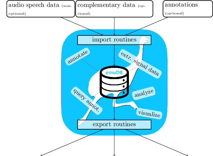
As the EMU-SDMS is not concerned with the raw data acquisition, other tools such as SpeechRecorder by Draxler and Jänsch (2004) are first used to record speech. However, once audio speech recordings are available, the system provides multiple conversion routines for converting existing collections of files to the new emuDB format described in Chapter 5 and importing them into the new EMU system. The current import routines provided by the emuR package are:
convert_TextGridCollection()- Convert TextGrid collections (.wavand.TextGridfiles) to theemuDBformat,convert_BPFCollection()- Convert Bas Partitur Format (BPF) collections (.wavand.parfiles) to theemuDBformat,convert_txtCollection()- Convert plain text file collections format (.wavand.txtfiles) to theemuDBformat,convert_legacyEmuDB()- Convert the legacy EMU database format to theemuDBformat andcreate_emuDB()followed byadd_link/levelDefinitionandimport_mediaFiles()- CreatingemuDBs from scratch with only audio files present.
The emuR package comes with a set of example files and small databases that are used throughout the emuR documentation, including the functions help pages. These can be accessed by typing help(function_name) or the short form ?function_name. R code snippet below illustrates how to create this demo data in a user-specified directory. Throughout the examples of this documentation the directory that is provided by the base R function tempdir() will be used, as this is available on every platform supported by R (see ?tempdir for further details). As can be inferred from the list.dirs() output in the below code, the emuR_demoData directory contains a separate directory containing example data for each of the import routines. Additionally, it contains a directory containing an emuDB called ae (the directories name is ae_emuDB, where _emuDB is the default suffix given to directories containing a emuDB; see Chapter 5).
# load the package
library(emuR)

# create demo data in directory provided by the tempdir() function
# (of course other directory paths may be chosen)
create_emuRdemoData(dir = tempdir())

# create path to demo data directory, which is
# called "emuR_demoData"
demo_data_dir = file.path(tempdir(), "emuR_demoData")

# show demo data directories
list.dirs(demo_data_dir, recursive = F, full.names = F)
## [1] "ae_emuDB" "BPF_collection" "legacy_ae"
## [4] "TextGrid_collection" "txt_collection"This tutorial will start by converting a TextGrid collection containing seven annotated single-sentence utterances of a single male speaker to the emuDB format3. In the EMU-SDMS, a file collection such as a TextGrid collection refers to a set of file pairs where two types of files with different file extentions are present (e.g., .ext1 and .ext2). It is vital that file pairs have the same basenames (e.g., A.ext1 and A.ext2 where A represents the basename) in order for the conversion functions to be able to pair up files that belong together. As other speech software tools also encourage such file pairs (e.g., Kisler et al. (2015)) this is a common collection format in the speech sciences. The R code snippet below shows such a file collection that is part of emuR’s demo data. Figure 3.1 shows the content of an annotation as displayed by Praat’s "Draw visible sound and Textgrid..." procedure.
# create path to TextGrid collection
tg_col_dir = file.path(demo_data_dir, "TextGrid_collection")

# show content of TextGrid_collection directory
list.files(tg_col_dir)
## [1] "msajc003.TextGrid" "msajc003.wav" "msajc010.TextGrid"
## [4] "msajc010.wav" "msajc012.TextGrid" "msajc012.wav"
## [7] "msajc015.TextGrid" "msajc015.wav" "msajc022.TextGrid"
## [10] "msajc022.wav" "msajc023.TextGrid" "msajc023.wav"
## [13] "msajc057.TextGrid" "msajc057.wav"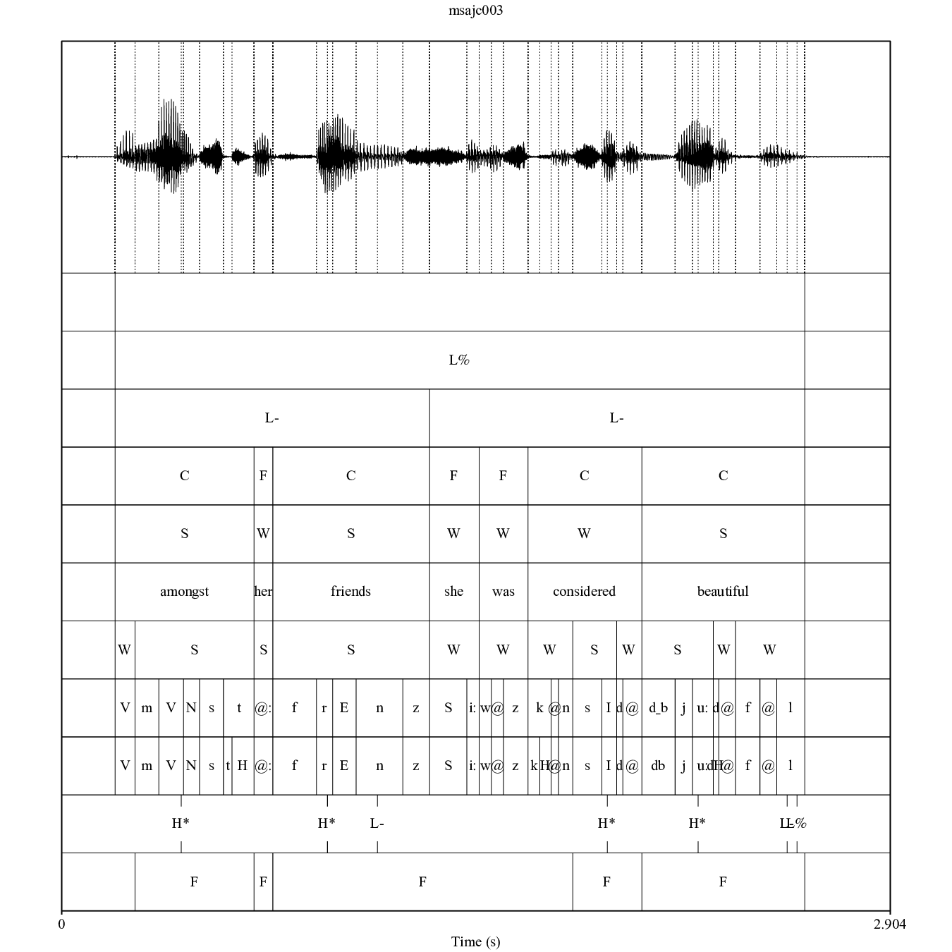
Figure 3.1: TextGrid annotation of the emuR_demoData/TextGrid_collection/msajc003.wav / .TextGrid file pair containing the tiers (from top to bottom): Utterance, Intonational, Intermediate, Word, Accent, Text, Syllable, Phoneme, Phonetic, Tone, Foot.
3.1 Converting the TextGrid collection
The convert_TextGridCollection() function converts a TextGrid collection to the emuDB format. A precondition that all .TextGrid files have to fulfill is that they must all contain the same tiers. If this is not the case, yet there is an equal tier subset that is contained in all the TextGrid files, this equal subset may be chosen. For example, if all .TextGrid files contain only the tier Phonetic: IntervalTier the conversion will work. However, if a single .TextGrid of the collection has the additional tier Tone: TextTier the conversion will fail. In this case the conversion could be made to work by specifying the equal subset (e.g., equalSubset = c("Phonetic")) and passing it on to the tierNames function argument convert_TextGridCollection(..., tierNames = equalSubset, ...). As can be seen in Figure 3.1, the TextGrid files provided by the demo data contain eleven tiers. To reduce the complexity of the annotations for this tutorial we will only convert the tiers Word (content: C vs. function: F word annotations), Syllable (strong: S vs. weak: W syllable annotations), Phoneme (phoneme level annotations) and Phonetic (phonetic annotations using Speech Assessment Methods Phonetic Alphabet (SAMPA) symbols - Wells and others (1997)) using the tierNames parameter. This conversion can be seen in the R code snippet below.
# convert TextGrid collection to the emuDB format
convert_TextGridCollection(dir = tg_col_dir,
                           dbName = "my-first",
                           targetDir = tempdir(),
                           tierNames = c("Word", "Syllable",
                                         "Phoneme", "Phonetic"))
The above call to convert_TextGridCollection() creates a new emuDB directory in the tempdir() directory called my-first_emuDB. This emuDB contains annotation files that contain the same Word, Syllable, Phoneme and Phonetic segment tiers as the original .TextGrid files as well as copies of the original (.wav) audio files. For further details about the structure of an emuDB, see Chapter 5 of this document.
3.2 Loading and inspecting the database
As mentioned in Section 2.2, the first step when working with an emuDB is to load it into the current R session. The R code snippet below shows how to load the converted TextGrid collection into R using the load_emuDB() function.
# get path to emuDB called "my-first"
# that was created by convert_TextGridCollection()
path2directory = file.path(tempdir(), "my-first_emuDB")

# load emuDB into current R session
# (verbose = F is only set to avoid additional output in manual)
db_handle = load_emuDB(path2directory,
                       verbose = FALSE)
3.2.1 Overview
Now the my-first emuDB is loaded into R, an overview of the current status and configuration of the database can be displayed using the summary() function as is shown by the below R code snippet.
# show summary
summary(db_handle)
## Name: my-first
## UUID: 31fbfcdc-deaa-4692-b05f-83e715e7de0d
## Directory: /tmp/RtmpXoGwEr/my-first_emuDB
## Session count: 1
## Bundle count: 7
## Annotation item count: 664
## Label count: 664
## Link count: 0
##
## Database configuration:
##
## SSFF track definitions:
## NULL
##
## Level definitions:
## name type nrOfAttrDefs attrDefNames
## 1 Word SEGMENT 1 Word;
## 2 Syllable SEGMENT 1 Syllable;
## 3 Phoneme SEGMENT 1 Phoneme;
## 4 Phonetic SEGMENT 1 Phonetic;
##
## Link definitions:
## NULLThe extensive output of summary() is split into a top and bottom half, where the top half focuses on general information about the database (name, directory, annotation item count, etc.) and the bottom half displays information about the various SSFF track, level and link definitions of the emuDB. The summary information about the level definitions shows, for instance, that the my-first database has a Word level of type SEGMENT and therefore contains annotation items that have a start time and a segment duration. It is worth noting that information about the SSFF track, level and link definitions corresponds to the output of the list_ssffTrackDefinitions(), list_levelDefinitions() and list_linkDefinitions() functions.
3.2.2 Database annotation and visual inspection
The EMU-SDMS has a unique approach to annotating and visually inspecting databases, as it utilizes a web application called the EMU-webApp to act as its GUI. To be able to communicate with the web application the emuR package provides the serve() function which is used in the R code snippet below.
# serve my-first emuDB to the EMU-webApp
serve(db_handle)
Executing this command will either automatically open up the system’s default browser or, if using RStudio, download the current EMU-webApp and display it in RStudio’s viewer pane and additionally display the following message in the R console:
## Navigate your browser to the EMU-webApp URL:
##  https://ips-lmu.github.io/EMU-webApp/ (should happen autom...
## Server connection URL:
##  ws://localhost:17890
## To stop the server either press the 'clear' button in the EMU-webApp,
##  close/reload the webApp in your browser,
## or call the httpuv::stopAllServers() function
The EMU-webApp, which is now connected to the database via the serve() function, can be used to visually inspect and annotate the emuDB. Figure 3.2 displays a screenshot of what the EMU-webApp looks like after automatically connecting to the server. As the EMU-webApp is a very feature-rich software annotation tool, this documentation has a whole chapter (see Chapter 9) on how to use it, what it is capable of and how to configure it. To close the connection and free up the blocked R console, simply click the clear button in the top menu bar of the EMU-webApp.
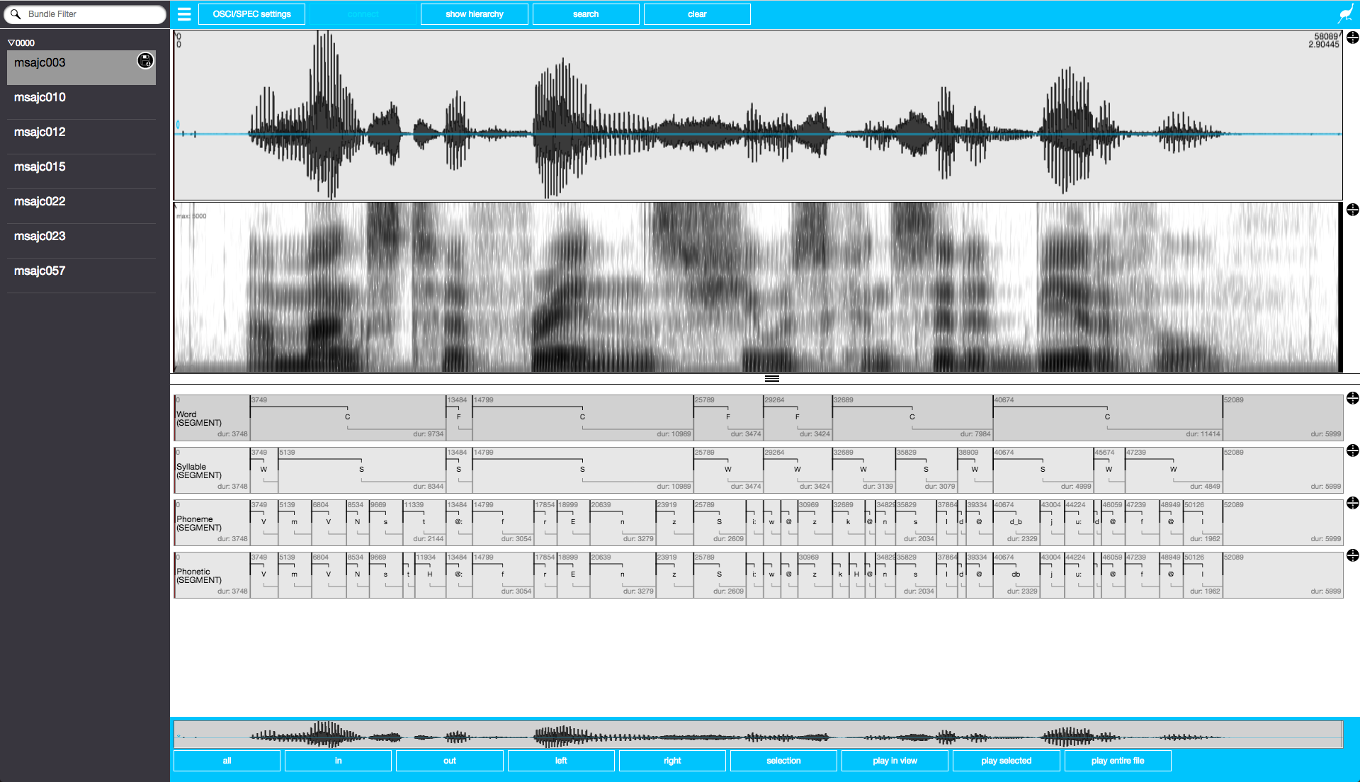
Figure 3.2: Screenshot of EMU-webApp displaying msajc003 bundle of my-first emuDB.
3.3 Querying and autobuilding the annotation structure
An integral step in the default workflow of the EMU-SDMS is querying the annotations of a database. The emuR package implements a query() function to accomplish this task. This function evaluates an EMU Query Language (EQL) expression and extracts the annotation items from the database that match a query expression. As chapter 6 gives a detailed description of the query mechanics provided by emuR, this tutorial will only use a very small, hopefully easy to understand subset of the EQL.
The output of the summary() command in the R code snippet below and the screenshot in Figure 3.2 show that the my-first emuDB contains four levels of annotations. The R code snippet below shows four separate queries that query various segments on each of the available levels. The query expressions all use the matching operator == which returns annotation items whose labels match those specified to the right of the operator and that belong to the level specified to the left of the operator (i.e., LEVEL == LABEL; see Chapter 6 for a detailed description).
# query all segments containing the label
# "C" (== content word) of the "Word" level
sl_text = query(emuDBhandle = db_handle,
                query = "Word == C")

# query all segments containing the label
# "S" (== strong syllable) of the "Syllable" level
sl_syl = query(emuDBhandle = db_handle,
               query = "Syllable == S")

# query all segments containing the label
# "f" on the "Phoneme" level
sl_phoneme = query(db_handle,
                   query = "Phoneme == f")

# query all segments containing the label
# "n" of the "Phonetic" level
sl_phonetic = query(db_handle,
                    query = "Phonetic == n")

# show class vector of query result
class(sl_phonetic)
## [1] "tbl_df" "tbl" "data.frame"# show first few entries of sl_phonetic
sl_phonetic## # A tibble: 12 x 16
## labels start end db_uuid session bundle start_item_id end_item_id level
## <chr> <dbl> <dbl> <chr> <chr> <chr> <int> <int> <chr>
## 1 n 1032. 1196. 31fbfc… 0000 msajc… 98 98 Phon…
## 2 n 1741. 1791. 31fbfc… 0000 msajc… 108 108 Phon…
## 3 n 1515. 1554. 31fbfc… 0000 msajc… 113 113 Phon…
## 4 n 2431. 2528. 31fbfc… 0000 msajc… 127 127 Phon…
## 5 n 895. 1023. 31fbfc… 0000 msajc… 98 98 Phon…
## 6 n 2402. 2475. 31fbfc… 0000 msajc… 122 122 Phon…
## 7 n 2227. 2271. 31fbfc… 0000 msajc… 132 132 Phon…
## 8 n 3046. 3068. 31fbfc… 0000 msajc… 145 145 Phon…
## 9 n 1435. 1495. 31fbfc… 0000 msajc… 91 91 Phon…
## 10 n 1775. 1834. 31fbfc… 0000 msajc… 96 96 Phon…
## 11 n 509. 544. 31fbfc… 0000 msajc… 97 97 Phon…
## 12 n 2448. 2480. 31fbfc… 0000 msajc… 130 130 Phon…
## # … with 7 more variables: attribute <chr>, start_item_seq_idx <int>,
## # end_item_seq_idx <int>, type <chr>, sample_start <int>, sample_end <int>,
## # sample_rate <int>As demonstrated in the above R code, the result of a query is a tbl_df object (i.e. a tibble object), which is a super-class of the common data.frame. For historical reasons the result of a query is often referred to as a segment list, or “seglist.” A segment list carries information about the extracted annotation items such as the extracted labels, the start and end times of the segments, the sessions and bundles the items are from and the levels they belong to. An in-depth description of the information contained in a segment list is given in Section 6.1.
3.4 Autobuilding
The simple queries illustrated above query segments from a single level that match a certain label. However, the EMU-SDMS offers a mechanism for performing inter-level queries such as: Query all Phonetic items that contain the label “n” and are part of a content word. For such queries to be possible, the EMU-SDMS offers very sophisticated annotation structure modeling capabilities, which are described in Chapter 4. For the sake of this tutorial we will focus on converting the flat segment level annotation structure displayed in Figure 3.2 to a hierarchical form as displayed in Figure 3.3, where only the Phonetic level carries time information and the annotation items on the other levels are explicitly linked to each other to form a hierarchical annotation structure.
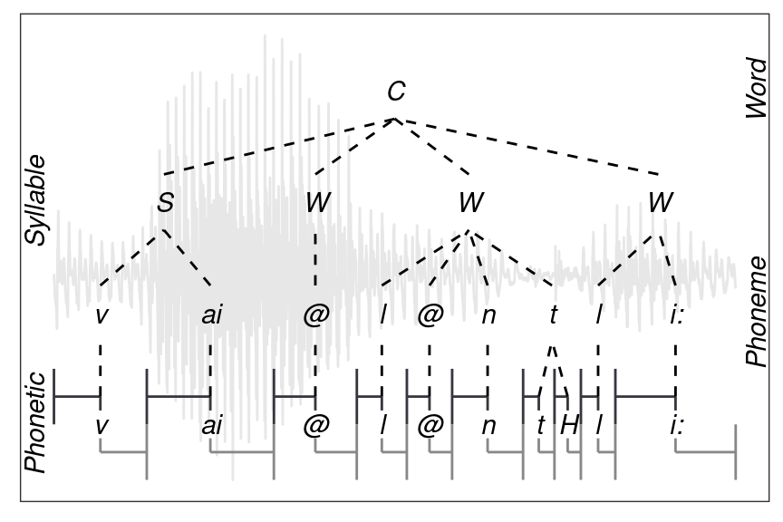
Figure 3.3: Example of a hierarchical annotation of the content (==C) word violently belonging to the msajc012 bundle of the my-first demo emuDB.
As it is a very laborious task to manually link annotation items together using the EMU-webApp and the hierarchical information is already implicitly contained in the time information of the segments and events of each level, we will now use a function provided by the emuR package to build these hierarchical structures using this information called autobuild_linkFromTimes(). The above R code snippet shows the calls to this function which autobuild the hierarchical annotations in the my-first database. As a general rule for autobuilding hierarchical annotation structures, a good strategy is to start the autobuilding process beginning with coarser grained annotation levels (i.e., the Word/Syllable level pair in our example) and work down to finer grained annotations (i.e., the Syllable/Phoneme and Phoneme/Phonetic level pairs in our example). To build hierachical annotation structures we need link definitions, which together with the level definitions define the annotation structure for the entire database (see Chapter 4 for further details). The autobuild_linkFromTimes() calls in the below R code snippet use the newLinkDefType parameter, which if defined automatically adds a link definition to the database.
# invoke autobuild function
# for "Word" and "Syllable" levels
autobuild_linkFromTimes(db_handle,
                        superlevelName = "Word",
                        sublevelName = "Syllable",
                        convertSuperlevel = TRUE,
                        newLinkDefType = "ONE_TO_MANY")

# invoke autobuild function
# for "Syllable" and "Phoneme" levels
autobuild_linkFromTimes(db_handle,
                        superlevelName = "Syllable",
                        sublevelName = "Phoneme",
                        convertSuperlevel = TRUE,
                        newLinkDefType = "ONE_TO_MANY")

# invoke autobuild function
# for "Phoneme" and "Phonetic" levels
autobuild_linkFromTimes(db_handle,
                        superlevelName = "Phoneme",
                        sublevelName = "Phonetic",
                        convertSuperlevel = TRUE,
                        newLinkDefType = "MANY_TO_MANY")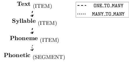
Figure 3.4: Schematic annotation structure of the emuDB after calling the autobuild function in R code snippet above.
As the autobuild_linkFromTimes() function automatically creates backup levels to avoid the accidental loss of boundary or event time information, the R code snippet below shows how these backup levels can be removed to clean up the database. However, using the remove_levelDefinition() function with its force parameter set to TRUE is a very invasive action. Usually this would not be recommended, but for this tutorial we are keeping everything as clean as possible.
# list level definitions
# as this reveals the "-autobuildBackup" levels
# added by the autobuild_linkFromTimes() calls
list_levelDefinitions(db_handle)
## name type nrOfAttrDefs attrDefNames
## 1 Word ITEM 1 Word;
## 2 Syllable ITEM 1 Syllable;
## 3 Phoneme ITEM 1 Phoneme;
## 4 Phonetic SEGMENT 1 Phonetic;
## 5 Word-autobuildBackup SEGMENT 1 Word-autobuildBackup;
## 6 Syllable-autobuildBackup SEGMENT 1 Syllable-autobuildBackup;
## 7 Phoneme-autobuildBackup SEGMENT 1 Phoneme-autobuildBackup;# remove the levels containing the "-autobuildBackup"
# suffix
# (verbose = F is only set to avoid additional output in manual)
remove_levelDefinition(db_handle,
name = "Word-autobuildBackup",
force = TRUE,
verbose = FALSE)
# (verbose = F is only set to avoid additional output in manual)
remove_levelDefinition(db_handle,
name = "Syllable-autobuildBackup",
force = TRUE,
verbose = FALSE)
# (verbose = F is only set to avoid additional output in manual)
remove_levelDefinition(db_handle,
name = "Phoneme-autobuildBackup",
force = TRUE,
verbose = FALSE)
# list level definitions
list_levelDefinitions(db_handle)## name type nrOfAttrDefs attrDefNames
## 1 Word ITEM 1 Word;
## 2 Syllable ITEM 1 Syllable;
## 3 Phoneme ITEM 1 Phoneme;
## 4 Phonetic SEGMENT 1 Phonetic;# list level definitions
# which were added by the autobuild functions
list_linkDefinitions(db_handle)## type superlevelName sublevelName
## 1 ONE_TO_MANY Word Syllable
## 2 ONE_TO_MANY Syllable Phoneme
## 3 MANY_TO_MANY Phoneme PhoneticAs can be seen by the output of list_levelDefinitions() and list_linkDefinitions() in the above R code, the annotation structure of the my-first emuDB now matches that displayed in Figure 3.4. Using the serve() function to open the emuDB in the EMU-webApp followed by clicking on the show hierarchy button in the top menu (and rotating the hierarchy by 90 degrees by clicking the rotate by 90 degrees button) will result in a view similar to the screenshot of Figure 3.5.
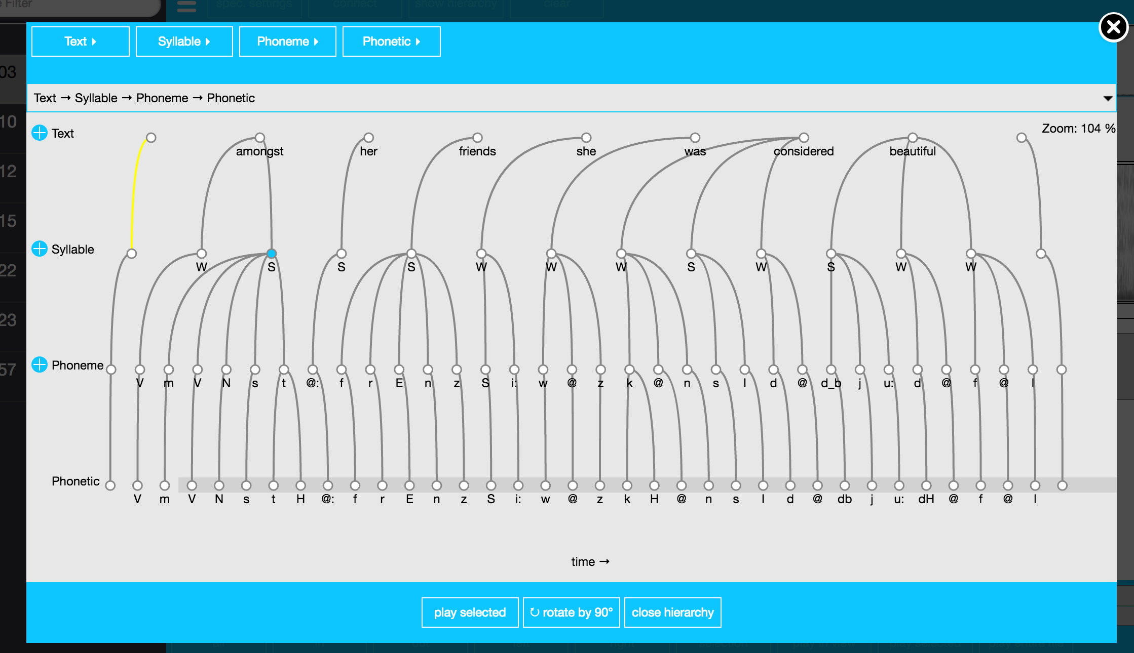
Figure 3.5: Screenshot of EMU-webApp displaying the autobuilt hierarchy of the my-first emuDB.
3.4.1 Querying the hierarchical annotations
Having this hierarchical annotation structure now allows us to formulate a query that helps answer the originally stated question: Given an annotated speech database, is the vowel height of the vowel @ (measured by its correlate, the first formant frequency) influenced by whether it appears in a content or function word?. The R code snippet below shows how all the @ vowels in the my-first database are queried.
# query annotation items containing
# the labels @ on the Phonetic level
sl_vowels = query(db_handle, "Phonetic == @")

# show sl_vowels
sl_vowels
## # A tibble: 28 x 16
## labels start end db_uuid session bundle start_item_id end_item_id level
## <chr> <dbl> <dbl> <chr> <chr> <chr> <int> <int> <chr>
## 1 @ 1506. 1548. 31fbfc… 0000 msajc… 103 103 Phon…
## 2 @ 1715. 1741. 31fbfc… 0000 msajc… 107 107 Phon…
## 3 @ 1967. 2034. 31fbfc… 0000 msajc… 112 112 Phon…
## 4 @ 2303. 2362. 31fbfc… 0000 msajc… 117 117 Phon…
## 5 @ 2447. 2506. 31fbfc… 0000 msajc… 119 119 Phon…
## 6 @ 1917. 1958. 31fbfc… 0000 msajc… 118 118 Phon…
## 7 @ 2022. 2078. 31fbfc… 0000 msajc… 120 120 Phon…
## 8 @ 2382. 2431. 31fbfc… 0000 msajc… 126 126 Phon…
## 9 @ 330. 380. 31fbfc… 0000 msajc… 91 91 Phon…
## 10 @ 1472. 1490. 31fbfc… 0000 msajc… 108 108 Phon…
## # … with 18 more rows, and 7 more variables: attribute <chr>,
## # start_item_seq_idx <int>, end_item_seq_idx <int>, type <chr>,
## # sample_start <int>, sample_end <int>, sample_rate <int>As the type of word (content vs. function) for each @ vowel is also needed, we can use the requery functionality of the EMU-SDMS (see Chapter 6) to retrieve the word type for each @ vowel. A requery essentially moves through a hierarchical annotation (vertically or horizontally) starting from the segments that are passed into the requery function. The R code below illustrates the usage of the hierarchical requery function, requery_hier(), to retrieve the appropriate annotation items from the Word level.
# hierarchical requery starting from the items in sl_vowels
# and moving up to the "Word" level
sl_word_type = requery_hier(db_handle,
                           seglist = sl_vowels,
                           level = "Word",
                           calcTimes = FALSE)

# show sl_word_type
sl_word_type
## # A tibble: 28 x 16
## labels start end db_uuid session bundle start_item_id end_item_id level
## <chr> <dbl> <dbl> <chr> <chr> <chr> <int> <int> <chr>
## 1 F NA NA 31fbfc… 0000 msajc… 16 16 Word
## 2 C NA NA 31fbfc… 0000 msajc… 17 17 Word
## 3 C NA NA 31fbfc… 0000 msajc… 17 17 Word
## 4 C NA NA 31fbfc… 0000 msajc… 18 18 Word
## 5 C NA NA 31fbfc… 0000 msajc… 18 18 Word
## 6 C NA NA 31fbfc… 0000 msajc… 19 19 Word
## 7 C NA NA 31fbfc… 0000 msajc… 20 20 Word
## 8 C NA NA 31fbfc… 0000 msajc… 20 20 Word
## 9 F NA NA 31fbfc… 0000 msajc… 13 13 Word
## 10 F NA NA 31fbfc… 0000 msajc… 17 17 Word
## # … with 18 more rows, and 7 more variables: attribute <chr>,
## # start_item_seq_idx <int>, end_item_seq_idx <int>, type <chr>,
## # sample_start <int>, sample_end <int>, sample_rate <int># show that sl_vowel and sl_word_type have the
# same number of row entries
nrow(sl_vowels) == nrow(sl_word_type)## [1] TRUEAs can be seen by the nrow() comparison in the above R code, the segment list returned by the requery_hier() function has the same number of rows as the original sl_vowels segment list. This is important, as each row of both segment lists line up and allow us to infer which segment belongs to which word type (e.g., vowel sl_vowels[5,] belongs to the word type sl_word_type[5,]).
3.5 Signal extraction and exploration
Now that the vowel and word type information including the vowel start and end time information has been extracted from the database, this information can be used to extract signal data that matches these segments. Using the emuR function get_trackdata() we can calculate the formant values in real time using the formant estimation function, forest(), provided by the wrassp package (see Chapter 8 for details). The following R code shows the usage of this function.
# get formant values for the vowel segments
# (verbose = F is only set to avoid additional output in manual)
td_vowels = get_trackdata(db_handle,
                          seglist = sl_vowels,
                          onTheFlyFunctionName = "forest",
                          verbose = F)

# show class vector
class(td_vowels)
## [1] "tbl_df" "tbl" "data.frame"# show dimensions
dim(td_vowels)## [1] 287 24# show nr of segments
max(td_vowels$sl_rowIdx)## [1] 28# display all values for fifth segment using dplyr
library(dplyr)
td_vowels %>% filter(sl_rowIdx == 5)## # A tibble: 12 x 24
## sl_rowIdx labels start end db_uuid session bundle start_item_id end_item_id
## <int> <chr> <dbl> <dbl> <chr> <chr> <chr> <int> <int>
## 1 5 @ 2447. 2506. 31fbfc… 0000 msajc… 119 119
## 2 5 @ 2447. 2506. 31fbfc… 0000 msajc… 119 119
## 3 5 @ 2447. 2506. 31fbfc… 0000 msajc… 119 119
## 4 5 @ 2447. 2506. 31fbfc… 0000 msajc… 119 119
## 5 5 @ 2447. 2506. 31fbfc… 0000 msajc… 119 119
## 6 5 @ 2447. 2506. 31fbfc… 0000 msajc… 119 119
## 7 5 @ 2447. 2506. 31fbfc… 0000 msajc… 119 119
## 8 5 @ 2447. 2506. 31fbfc… 0000 msajc… 119 119
## 9 5 @ 2447. 2506. 31fbfc… 0000 msajc… 119 119
## 10 5 @ 2447. 2506. 31fbfc… 0000 msajc… 119 119
## 11 5 @ 2447. 2506. 31fbfc… 0000 msajc… 119 119
## 12 5 @ 2447. 2506. 31fbfc… 0000 msajc… 119 119
## # … with 15 more variables: level <chr>, attribute <chr>,
## # start_item_seq_idx <int>, end_item_seq_idx <int>, type <chr>,
## # sample_start <int>, sample_end <int>, sample_rate <int>, times_orig <dbl>,
## # times_rel <dbl>, times_norm <dbl>, T1 <int>, T2 <int>, T3 <int>, T4 <int>As can be seen by the call to the class() function, the resulting object is of the type tibble (see ?tibble::tibble for more information) and has 28 blocks of data. These blocks correspond to the number of rows contained in the segment lists extracted above (i.e., nrow(sl_vowels)) and can be matched to the according segment using the sl_rowIdx column (i.e., td_vowels %>% filter(sl_rowIdx == 5) are the formant values belonging to sl_vowels[5,]). As the columns T1, T2, T3, T4 of the printed output of td_vowels %>% filter(sl_rowIdx == 5) suggest, the forest function estimates four formant values. We will only be concerned with the first (column T1) and second (column T2). The below R code shows two ggplot() function calls which produce the plots displayed in Figures 3.6 and 3.6. The first ggplot() call plots all 28 first formant trajectories (achieved by setting the group parameter to sl_rowIdx). To clean up the cluttered first plot, the second ggplot() call uses a segment length normalized version of td_vowels (see ?normalize_length for futher details) as well as using geom_smooth() in combination with setting the group parameter to labels to plot only smoothed conditional means of all @ vowels.
# load package
library(ggplot2)

ggplot(td_vowels) +
  aes(x = times_rel, y = T1, col = labels, group = sl_rowIdx) +
  geom_line() +
  labs(x = "Duration (ms)", y = "F1 (Hz)")

# normalize length of segments
td_vowels_norm = normalize_length(td_vowels)

ggplot(td_vowels_norm) +
  aes(x = times_norm, y = T1, col = labels, group = labels) +
  geom_smooth() +
labs(x = "Duration (normalized)", y = "F1 (Hz)") 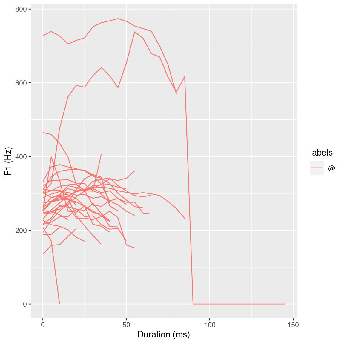
Figure 3.6: ggplot() plots of all F1 @ vowel trajectories.
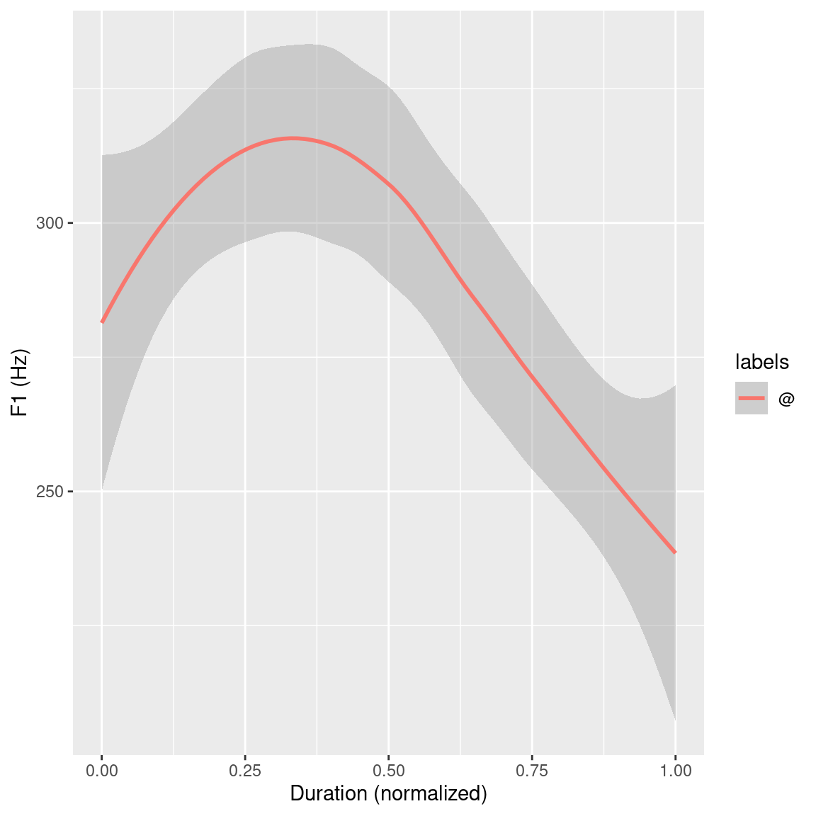
Figure 3.7: ggplot() plots of the F1 smoothed conditional mean trajectories of all @ vowels.
Figures 3.6 and 3.7 give an overview of the first formant trajectories of the @ vowels. For the purpose of data exploration and to get an idea of where the individual vowel classes lie on the F2 x F1 plane, which indirectly provides information about vowel height and tongue position, the R code below again makes use of the ggplot() function. This produces Figure 3.8. To be able to use the stat_ellipse() function, the td_vowels_norm object first has to be modified, as it contains entire formant trajectories but two dimensional data is needed to be able to display it on the F2 x F1 plain. This can, for example, be achieved by only extracting temporal mid-point formant values for each vowel using the get_trackdata() function utilizing its cut parameter. The R code snippet below shows an alternative approach using the dplyr’s filter() function to essentially cut the formant trajectories to a specified proportional segment. By only extracting the values that have a normalized time value of 0.5 (times_norm == 0.5) only the formant values that are at the time normalized mid-point (calculated above using the normalize_length() function) are extracted from the trajectories.
# cut formant trajectories at temporal mid-point
td_vowels_midpoint = td_vowels_norm %>%
  filter(times_norm == 0.5)

# show dimensions of td_vowels_midpoint
dim(td_vowels_midpoint)

# calculate centroid
td_centroids = td_vowels_midpoint %>%
  group_by(labels) %>%
  summarise(T1 = mean(T1), T2 = mean(T2))

# generate plot
ggplot(td_vowels_midpoint, aes(x = T2, y = T1, colour = labels, label = labels)) +
  geom_text(data = td_centroids) +
  stat_ellipse() +
  scale_y_reverse() + scale_x_reverse() +
  labs(x = "F2 (Hz)", y = "F1 (Hz)") +
  theme(legend.position="none")
## [1] 28 24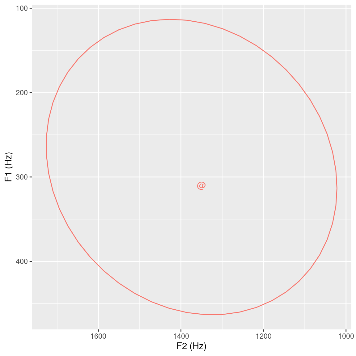
Figure 3.8: 95% ellipse plot including centroid for F2 x F1 data extracted from the temporal midpoint of the vowel segments.
Figure 3.8 displays the first two formants extracted at the temporal midpoint of every @ vowel in sl_vowels. The centroid of these formants is plotted on the F2 x F1 plane, and their 95% ellipsis distribution is also shown. Although not necessarily applicable to the question posed at the beginning of this tutorial, the data exploration using the dplyr and ggplot2 packages can be very helpful tools for providing an overview of the data at hand.
3.6 Vowel height as a function of word types (content vs. function): evaluation and statistical analysis
The above data exploration only dealt with the actual @ vowels and disregarded the syllable type they occurred in. However, the question in the introduction of this chapter focuses on whether the @ vowel occurs in a content (labeled C) or function (labeled F) word. For data inspection purposes, the R code snippet below initially extracts the central 60% (filter() conditions times_norm >= 0.2 and times_norm <= 0.8) of the formant trajectories from td_vowels_norm using dplyr and displays them using ggplot(). It should be noted that before the call to ggplot() the labels of the td_vowels_mid_sec are replaced with those of sl_word_type. This allows ggplot() to group the trajectories by their word type as opposed to their vowel labels as displayed in Figure 3.9.
# extract central 60% from formant trajectories
td_vowels_mid_sec = td_vowels_norm %>%
  filter(times_norm >= 0.2, times_norm <= 0.8)

# replace labels with those of sl_word_type
td_vowels_mid_sec$labels = sl_word_type$labels[td_vowels_mid_sec$sl_rowIdx]

ggplot(td_vowels_mid_sec) +
  aes(x = times_norm, y = T1, col = labels, group = labels) +
  geom_smooth() +
  labs(x = "Duration (normalized)", y = "F1 (Hz)")
## `geom_smooth()` using method = 'loess' and formula 'y ~ x'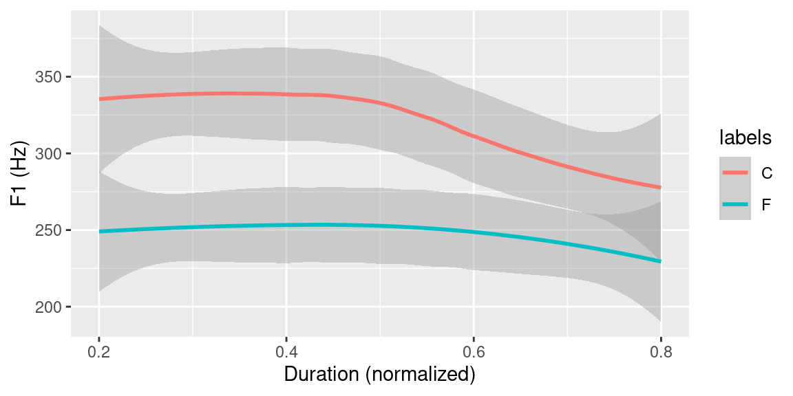
Figure 3.9: Ensemble averages of F1 contours of all tokens of the central 60% of vowels grouped by word type (function (F) vs. content (W)).
As can be seen in Figure 3.9, there seems to be a distinction in F1 trajectory height between vowels in content and function words. The following R snippet shows the code to produce a boxplot once again using the ggplot2 package to further visually inspect the data (see Figure 3.10 for the plot produced by the below code).
# use group_by + summarise to calculate the means of the 60%
# formant trajectories
td_vowels_mid_sec_mean = td_vowels_mid_sec %>%
  group_by(sl_rowIdx) %>%
  summarise(labels = unique(labels), meanF1 = mean(T1))


# create boxplot using ggplot
ggplot(td_vowels_mid_sec_mean, aes(labels, meanF1)) +
  geom_boxplot() +
  labs(x = "Word type", y = "mean F1 (Hz)")
## `summarise()` ungrouping output (override with `.groups` argument)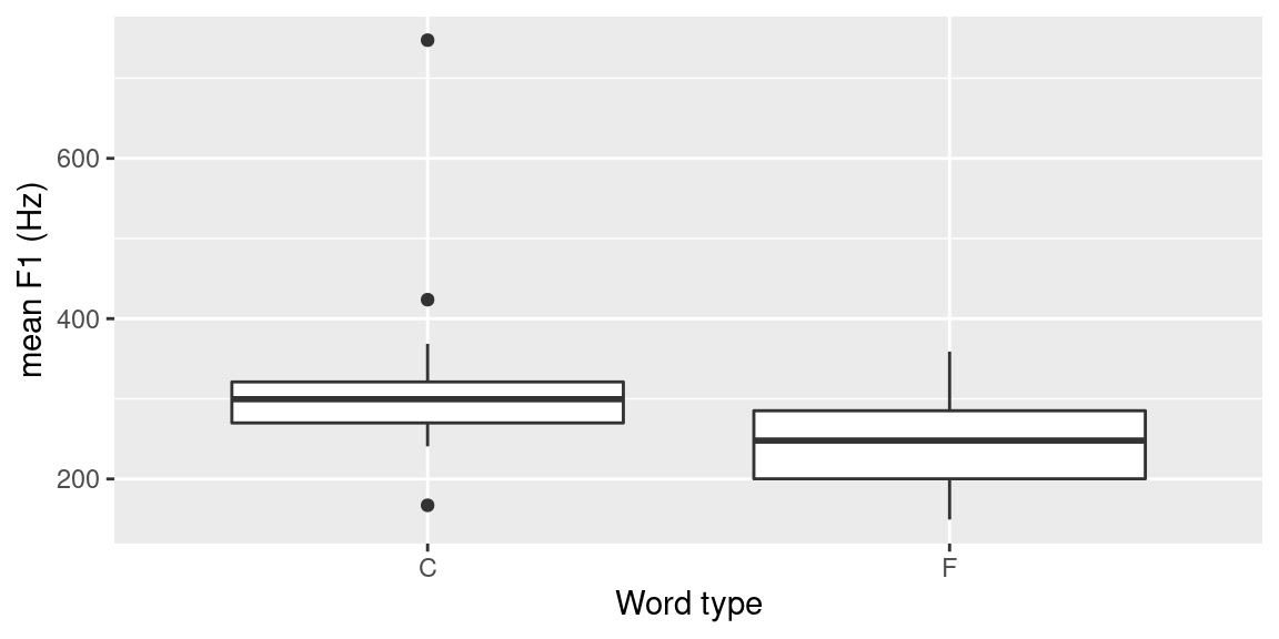
Figure 3.10: Boxplot produced using ggplot2 to visualize the difference in F1 depending on whether the vowel occurs in content (C) or function (F) word.
To confirm or reject this, the following R code presents a very simple statistical analysis of the F1 mean values of the 60% mid-section formant trajectories.4 First, a Shapiro-Wilk test for normality of the distributions of the F1 means for both word types is carried out. As only one type is normally distributed, a Wilcoxon rank sum test is performed. The density distributions (commented out plot() function calls in the code below) are displayed in Figure 3.11.
# calculate density for vowels in function words
distrF = density(td_vowels_mid_sec_mean[td_vowels_mid_sec_mean$labels == "F",]$meanF1)

# uncomment to visualize distribution
# plot(distrF)

# check that vowels in function
# words are normally distributed
shapiro.test(td_vowels_mid_sec_mean[td_vowels_mid_sec_mean$labels == "F",]$meanF1)
##
## Shapiro-Wilk normality test
##
## data: td_vowels_mid_sec_mean[td_vowels_mid_sec_mean$labels == "F", ]$meanF1
## W = 0.98618, p-value = 0.9868# p-value > 0.05 implying that the distribution
# of the data ARE NOT significantly different from
# normal distribution -> we CAN assume normality
# calculate density for vowels in content words
distrC = density(td_vowels_mid_sec_mean[td_vowels_mid_sec_mean$labels == "C",]$meanF1)
# uncomment to visualize distribution
# plot(distrC)
# check that vowels in content
# words are normally distributed:
shapiro.test(td_vowels_mid_sec_mean[td_vowels_mid_sec_mean$labels == "C",]$meanF1)##
## Shapiro-Wilk normality test
##
## data: td_vowels_mid_sec_mean[td_vowels_mid_sec_mean$labels == "C", ]$meanF1
## W = 0.67216, p-value = 1.819e-05# p-value < 0.05 implying that the distribution
# of the data ARE significantly different from
# normal distribution -> we CAN NOT assume normality
# (this somewhat unexpected result is probably
# due to the small sample size used in this toy example)
# -> use Wilcoxon rank sum test
# perform Wilcoxon rank sum test to establish
# whether vowel F1 depends on word type
wilcox.test(meanF1 ~ labels, data = td_vowels_mid_sec_mean)##
## Wilcoxon rank sum exact test
##
## data: meanF1 by labels
## W = 119, p-value = 0.04875
## alternative hypothesis: true location shift is not equal to 0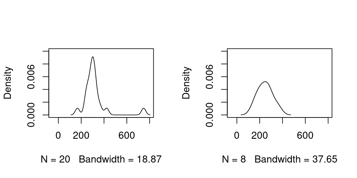
Figure 3.11: Plots of density distributions of vowels in content words (left plot) and vowels in function words (right plot) of the above R code.
As shown by the result of wilcox.test() in the above R code, word type (C vs. F) has a significant influence on the vowel’s F1 (W=121, p<0.05). Hence, the answer to the initially proposed question: Given an annotated speech database, is vowel height of the vowel @ (measured by its correlate, the first formant frequency) influenced by whether it appears in a content or function word? is yes!
3.7 Conclusion
The tutorial given in this chapter gave an overview of what it is like working with the EMU-SDMS to try to solve a research question. As many of the concepts were only briefly explained, it is worth noting that explicit explanations of the various components and integral concepts are given in following chapters. Further, additional use cases that have been taken from the emuR_intro vignette can be found in Appendix 14. These use cases act as templates for various types of research questions and will hopefully aid the user in finding a solution similar to what she or he wishes to achieve.
Some examples of this chapter are adapted versions of examples of the
emuR_introvignette.↩︎The other input routines are covered in the Section @ref(sec:emuRpackageDetails_importRoutines).↩︎
It is worth noting that the sample size in this toy example is quite small. This obviously influences the outcome of the simple statistical analysis that is performed here.↩︎