9 The EMU-webApp¹⁶

The EMU-SDMS has a unique approach to its graphical user interface (GUI) in that it utilizes a web application as its primary GUI. This is known as the EMU-webApp . The EMU-webApp is a fully fledged browser-based labeling and correction tool that offers a multitude of labeling and visualization features. These features include unlimited undo/redo, formant correction capabilities, the ability to snap a preselected boundary to the nearest top/bottom boundary, snap a preselected boundary to the nearest zero crossing, and many more. The web application is able to render everything directly in the user’s browser, including the calculation and rendering of the spectrogram, as it is written entirely using HTML, CSS and JavaScript. This means it can also be used as a standalone labeling application, as it does not require any server-side calculations or rendering. Further, it is designed to interact with any websocket server that implements the EMU-webApp websocket protocol (see Section 13.1). This enables it to be used as a labeling tool for collaborative annotation efforts. Also, as the EMU-webApp is cached in the user’s browser on the first visit, it does not require any internet connectivity to be able to access the web application unless the user explicitly clears the browser’s cache. The URL of the current live version of the EMU-webApp is: http://ips-lmu.github.io/EMU-webApp/.

9.1 Main layout

The main screen of the EMU-webApp can be split into five areas. Figure 9.1 shows a screenshot of the EMU-webApp’s main screen displaying these five areas while displaying a bundle of the ae demo database. This database is served to the EMU-webApp by invoking the serve() command as shown in the R code snippet below. The left side bar (area marked 1 in Figure 9.1) represents the bundle list side bar which, if connected to a database, displays the currently available bundles grouped by their sessions. The top and bottom menu bars (areas marked 2 and 5 in Figure 9.1) display the currently available menu options, where the bottom menu bar contains the audio navigation and playback controls and also includes a scrollable mini map of the oscillogram. Area 3 of Figure 9.1 displays the signal canvas area currently displaying the oscillogram and the spectrogram. Other signal contours such as formant frequency contours and fundamental frequency contours are also displayed in this area. Area 4 of Figure 9.1 displays the area in which levels containing time information are displayed. It is worth noting that the main screen of the EMU-webApp does not display any levels that do not contain time information. The hierarchical annotation can be displayed and edited by clicking the show hierarchy button in the top menu bar (see Figure 9.6 for an example of how the hierarchy is displayed).

# serve ae emuDB to EMU-webApp
serve(ae)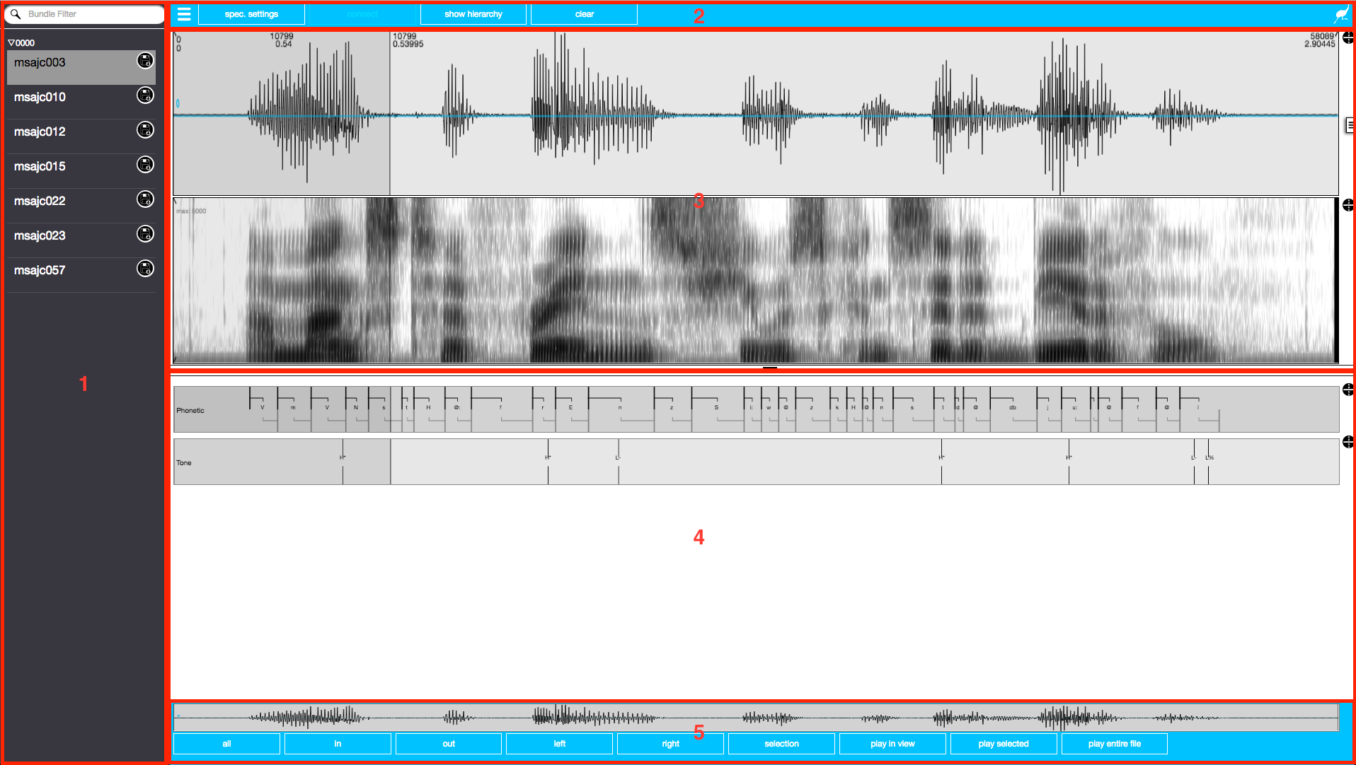

Figure 9.1: Screenshot of EMU-webApp displaying the ae demo database with overlaid areas of the main screen of the web application (see text).

9.2 General usage

This section introduces the labeling mechanics and general labeling workflow of the EMU-webApp. The EMU-webApp makes heavy use of keyboard shortcuts. Is is worth noting that most of the keyboard shortcuts are centered around the WASD keys, which are the navigation shortcut keys (W to zoom in; S to zoom out; A to move left and D to move right). For a full list of the available keyboard shortcuts see the EMU-webApp’s own manual, which can be accessed by clicking the EMU icon on the right hand side of the top menu bar (area 2 in Figure 9.1).

9.2.1 Annotating levels containing time information

Boundaries and events

The EMU-webApp has slightly different labeling mechanics compared with other annotation software. Compared to the usual click and drag of segment boundaries and event markers, the web application continuously tracks the movement of the mouse in levels containing time information, highlighting the boundary or event marker that is closest to it by coloring it blue. Figure 9.2 displays this automatic boundary preselection.

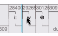
Figure 9.2: Screenshot of segment level as displayed by the EMU-webApp with superimposed mouse cursor displaying the automatic boundary preselection of closest boundary (boundary marked blue).

Once a boundary or event is preselected, the user can perform various actions with it. She or he can, for example, grab a preselected boundary or event by holding down the SHIFT key and moving it to the desired position, or delete the current boundary or event by hitting the BACKSPACE key. Other actions that can be performed on preselected boundaries or events are:

• snap to closest boundary or event in level above (Keyboard Shortcut t),
• snap to closest boundary or event in level below (Keyboard Shortcut b), and
• snap to nearest zero crossing (Keyboard Shortcut x).

To add a new boundary or event to a level the user initially has to select the desired level she or he wishes to edit. This is achieved either by using the up and down cursor keys or by single-left-clicking on the desired level. The current preselected level is marked in a darker shade of gray, as is displayed in Figure 9.3.

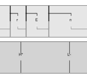
Figure 9.3: Screenshot of two levels as displayed by the EMU-webApp, where the lower level is preselected (i.e., marked in a darker shade of gray).

To add a boundary to the currently selected level one first has to select a point in time either in the spectrogram or the oscillogram by single-left-clicking on the desired location. Hitting the enter/return key adds a new boundary or event to the preselected level at the selected time point. Selecting a stretch of time in the spectrogram or the oscillogram (left-click-and-drag) and hitting enter will add a segment (not a boundary) to a preselected segment level.

Segments and events

The EMU-webApp also allows segments and events to be preselected by single-left-clicking the desired item. The web application colors the preselected segments and events yellow to indicate their pre-selection as displayed in Figure 9.4.

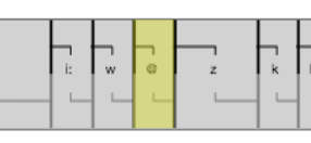
Figure 9.4: Screenshot of level as displayed by the EMU-webApp, where the /@/ segment is currently preselected as it is marked yellow.

As with preselected boundaries or events the user can now perform multiple actions with these preselected items. She or he can, for example, edit the item’s label by hitting the enter/return key (which can also be achieved by double-left-clicking the item). Other actions that can be performed on preselected items are:

• Select next item in level (keyboard shortcut TAB),
• Select previous item in level (keyboard shortcut SHIFT plus TAB),
• Add time to selected item(s) end (keyboard shortcut +),
• Add time to selected item(s) start (keyboard shortcut SHIFT plus +),
• Remove time to selected item(s) end (keyboard shortcut -),
• Remove time to selected item(s) start (keyboard shortcut SHIFT plus -), and
• Move selected item(s) (hold down ALT Key and drag to desired position).

By right-clicking adjacent segment or events (keyboard shortcut SHIFT plus left or right cursor keys), it is possible to select multiple items at once.

Parallel labels in segments and events

If a level containing time information has multiple attribute definitions (i.e., multiple parallel labels per segment or event) the EMU-webApp automatically displays radio buttons underneath that level (see red square in Figure 9.5) that allow the user to switch between the parallel labels. Figure 9.5 displays a segment level with three attribute definitions.

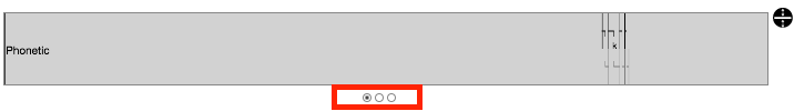
Figure 9.5: Screenshot of segment level with three attribute definitions. The radio buttons that switch between the parallel labels are highlighted by a red square.

Legal labels

As mentioned in Section 5.2.3.2, an array of so-called legal labels can be defined for every level or, more specifically, for each attribute definition. The EMU-webApp enforces these legal labels by not allowing any other labels to be entered in the label editing text fields. If an illegal label is entered, the text field will turn red and the EMU-webApp will not permit this label to be saved.

9.2.2 Working with hierarchical annotations¹⁷

Viewing the hierarchy

As mentioned in Section 9.1, pressing the show hierarchy button (keyboard shortcut h) in the top menu bar opens the hierarchy view modal window. As with most modal windows in the EMU-webApp, it can be closed by clicking on the close button, clicking the X circle icon in the top right hand corner of the modal or by hitting the ESCAPE key. By default, the hierarchy modal window displays a horizontal version of the hierarchy for a spatially economical visualization. As most people are more familiar with a vertical hierarchical annotation display, the hierarchy can be rotated by hitting the rotate by 90° button (keyboard shortcut r). Zooming in and out of the hierarchy can be achieved by using the mouse wheel, and moving through the hierarchy in time can be achieved by holding down the left mouse button and dragging the hierarchy in the desired direction. Figure 9.6 shows the hierarchy modal window displaying the hierarchical annotation of a single path (Utterance -> Intonational -> Intermediate -> Word -> Syllable -> Phoneme -> Phonetic) through a multi-path hierarchy of the ae emuDB in its horizontal form.

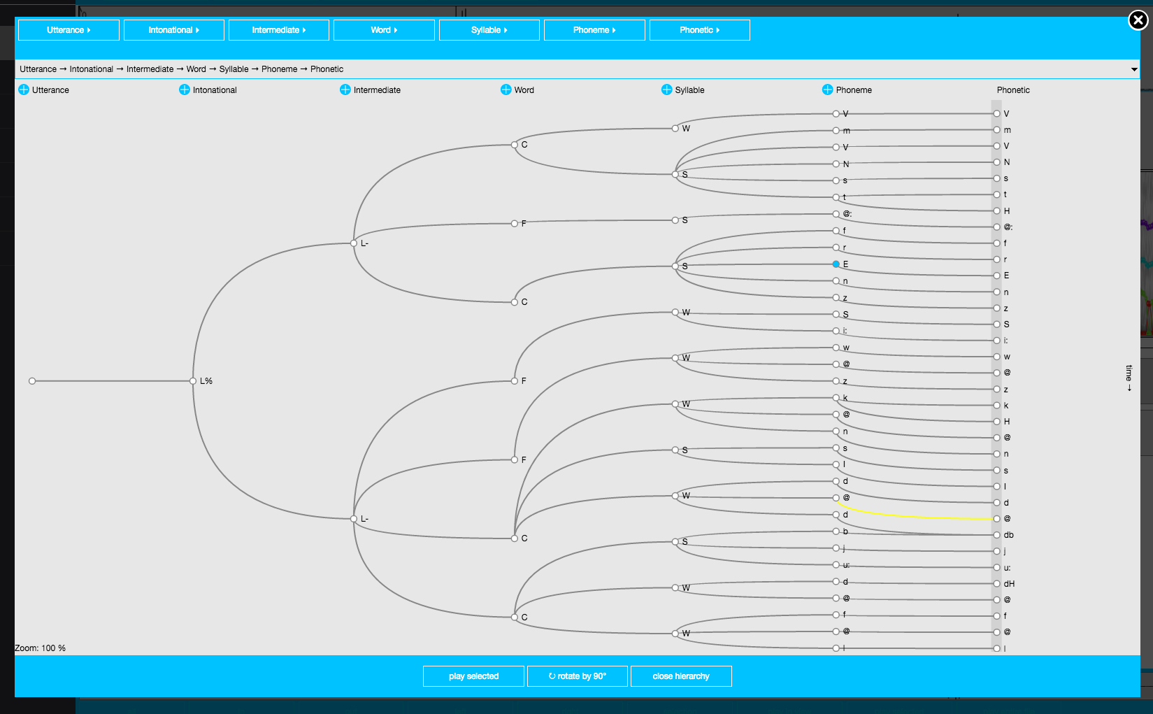
Figure 9.6: Screenshot of the hierarchy modal window level displaying a path through the hierarchy of the ae emuDB in its horizontal form.

Selecting a path through the hierarchy

As more complex databases have multiple hierarchical paths through their hierarchical annotation structure (see Figure 4.2B for an example of a multi-dimensional hierarchical annotation structure), the hierarchy modal offers a drop-down menu to choose the current path to be displayed. Area 2 in Figure 9.7 marks the hierarchy path drop-down menu of the hierarchy modal.

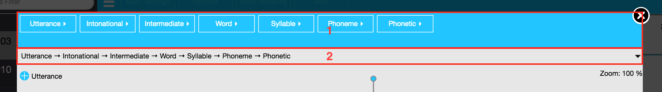
Figure 9.7: Screenshot of top of hierarchy modal window of the EMU-webApp in which the area marked 1 shows the drop-down menus for selecting the parallel label for each level and area 2 marks the hierarchy path drop-down menu.

It is worth noting that only non-partial paths can be selected in the hierarchy path drop-down menu.

Selecting parallel labels in timeless levels

As timeless levels may also contain multiple parallel labels, the hierarchy path modal window provides a drop-down menu for each level to select which label or attribute definition is to be displayed. Area 1 of Figure 9.7 displays these drop-down menus.

Adding a new item

The hierarchy modal window provides two methods for adding new annotation items to a level. This can either be achieved by pressing the blue and white + button next to the level’s name (which appends a new item to the end of the level) or by preselecting an annotation item (by hovering the mouse over it) and hitting either the n (insert new item before preselected item) or the m key (insert new item after preselected item).

Modifying an annotation item

An item’s context menu¹⁸ is opened by single-left-clicking its node. The resulting context menu displays a text area in which the label of the annotation item can be edited, a play button to play the audio section associated with the item and a collapse arrow button allowing the user to collapse the sub-tree beneath the current item. Collapsing a sub-tree can be useful for masking parts of the hierarchy while editing. A screenshot of the context menu is displayed in Figure 9.8.

Figure 9.8: Screenshot of the hierarchy modal window of the EMU-webApp displaying an annotation item’s context menu.

Adding a new link

Adding a new link between two items can be achieved by hovering the mouse over one of the two items, holding down the SHIFT key and moving the mouse cursor to the other item. A green dashed line indicates that the link to be added is valid, while a red dashed line indicates it is not. A link’s validity is dependent on the database’s configuration (i.e., if there is a link definition present and the type of link definition) as well as the non-crossing constraint (Coleman and Local 1991) that essentially implies that links are not allowed to cross each other. If the link is valid (i.e., a green dashed line is present), releasing the SHIFT key will add the link to the annotation.

Deleting an annotation item or a link

Items and links are deleted by initially preselecting them by hovering the mouse cursor over them. The preselected items are marked blue and preselected links yellow. A preselected link is removed by hitting BACKSPACE and a preselected item is deleted by hitting the y key. Deleting an item will also delete all links leading to and from it.

9.3 Configuring the EMU-webApp

This section will give an overview of how the EMU-webApp can be configured. The configuration of the EMU-webApp is stored in the EMUwebAppConfig section of the _DBconfig.json of an emuDB (see Appendix 15.1.1 for details). This means that the EMU-webApp can be configured separately for every emuDB. Although it can be necessary for some advanced configuration options to manually edit the _DBconfig.json using a text editor (see Section 9.3.3), the most common configuration operations can be achieved using functions provided by the emuR package (see Section 9.3.1).

A central concept for configuring the EMU-webApp are so-called perspectives. Essentially, a perspective is an independent configuration of how the EMU-webApp displays a certain set of data. Having multiple perspectives allows the user to switch between different views of the data. This can be especially useful when dealing with complex annotations where only showing certain elements for certain labeling tasks can be beneficial. Figure 9.9 displays a screenshot of the perspectives side bar menu of the EMU-webApp which displays the three perspectives of the ae emuDB¹⁹. The default perspective displays both the Phonetic and the Tone levels where as the Phonetic-only and the Tone-only only display these levels individually.

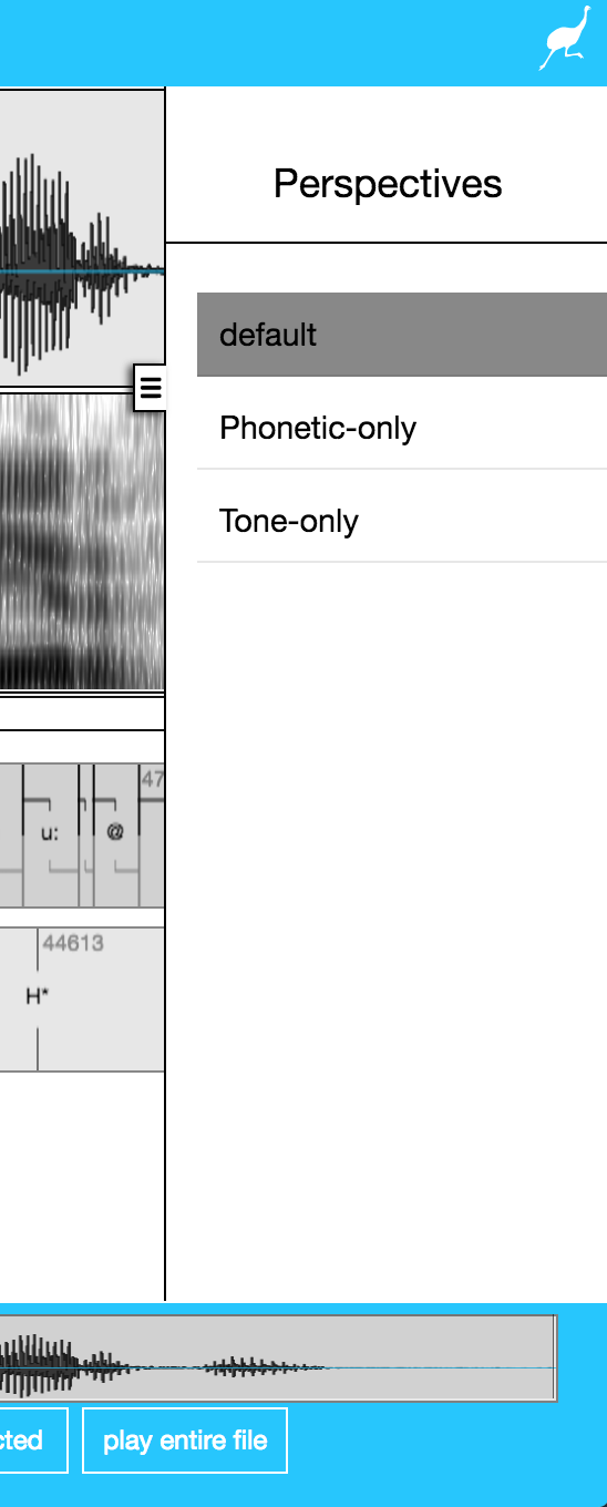
Figure 9.9: Screenshot of the hierarchy modal window of the EMU-webApp displaying an annotation item’s context menu.

9.3.1 Basic configurations using emuR

The R code snippet below shows how to create and load the demo data that will be used throughout the rest of this chapter.

# load package
library(emuR)

# create demo data in directory provided by tempdir()
create_emuRdemoData(dir = tempdir())

# create path to demo database
path2ae = file.path(tempdir(), "emuR_demoData", "ae_emuDB")

# load database
# (verbose = F is only set to avoid additional output in manual)
ae = load_emuDB(path2ae, verbose = F)

As mentioned above, the EMU-webApp subdivides different ways to look at an emuDB into so-called perspectives. Users can switch between these perspectives in the web application. They contain, for example, information on what levels are displayed, which SSFF tracks are drawn. The R code snippet below shows how the current perspectives can be listed using the list_perspectives() function.

# list perspectives of ae emuDB
list_perspectives(ae)

##            name signalCanvasesOrder levelCanvasesOrder
## 1       default          OSCI; SPEC     Phonetic; Tone
## 2 Phonetic-only          OSCI; SPEC           Phonetic
## 3     Tone-only          OSCI; SPEC               Tone

As it is sometimes necessary to add new or remove existing perspectives to or from a database, the R code snippet below shows how this can be achieved using emuR’s add/remove_perspective() functions.

# add new perspective to ae emuDB
add_perspective(ae,
                name = "tmp-persp")

# show added perspective
list_perspectives(ae)

##            name signalCanvasesOrder levelCanvasesOrder
## 1       default          OSCI; SPEC     Phonetic; Tone
## 2 Phonetic-only          OSCI; SPEC           Phonetic
## 3     Tone-only          OSCI; SPEC               Tone
## 4     tmp-persp          OSCI; SPEC

# remove newly added perspective
remove_perspective(ae,
                   name = "tmp-persp")

9.3.2 Signal canvas and level canvas order

As already mentioned, the above R code snippet shows that the ae emuDB contains three perspectives. The first perspective (default) displays the oscillogram (OSCI) followed by the spectrogram (SPEC) in the signal canvas area (area 3 of Figure 9.1) and the Phonetic and Tone levels in the level canvas area (area 4 of Figure 9.1). It is worth noting that OSCI (oscillogram) and SPEC (spectrogram) are predefined signal tracks that are always available. This is indicated by the capital letters indicating that they are predefined constants. The R code snippet below shows how the order of the signal canvases and level canvases can be changed using the get/set_signalCanvasesOrder() and get/set_levelCanvasesOrder().

# get order vector of signal canvases of default perspective
sco = get_signalCanvasesOrder(ae,
                              perspectiveName = "default")

# show sco vector
sco

## [1] "OSCI" "SPEC"

# reverse sco order
# using R's rev() function
scor = rev(sco)

# set order vector of signal canvases of default perspective
set_signalCanvasesOrder(ae,
                        perspectiveName = "default",
                        order = scor)

# set order vector of level canvases of default perspective
# to only display the "Tone" level
set_levelCanvasesOrder(ae,
                       perspectiveName = "default",
                       order = c("Tone"))

# list perspectives of ae emuDB
# to show changes
list_perspectives(ae)

##            name signalCanvasesOrder levelCanvasesOrder
## 1       default          SPEC; OSCI               Tone
## 2 Phonetic-only          OSCI; SPEC           Phonetic
## 3     Tone-only          OSCI; SPEC               Tone

After the changes made in the R code snippet above, the default perspective will show the spectrogram above the oscillogram in the signal canvas area and only the Tone level in the level canvas area. Only levels with time information are allowed to be displayed in the level canvas area, and the set_levelCanvasesOrder() will print an error if a level of type ITEM is added (see R code snippet below).

# set level canvas order where a
# level is passed into the order parameter
# that is not of type EVENT or SEGMENT
set_levelCanvasesOrder(ae,
                       perspectiveName = "default",
                       order = c("Syllable"))

## Error in set_levelCanvasesOrder(ae, perspectiveName = "default", order = c("Syllable")): levelDefinition with name 'Syllable' is not of type 'SEGMENT' or 'EVENT'

The same mechanism used above can also be used to display any SSFF track that is defined for the database by referencing its name. The R code snippet below shows how the existing SSFF track called fm (containing formant values calculated by wrassp’s forest() function) can be added to the signal canvas area.

# show currently available SSFF tracks
list_ssffTrackDefinitions(ae)

##   name columnName fileExtension
## 1  dft        dft           dft
## 2   fm         fm           fms

# re-set order vector of signal canvases of default perspective
# by appending the fm track
set_signalCanvasesOrder(ae,
                        perspectiveName = "default",
                        order = c(scor, "fm"))

A screenshot of the current display of the default perspective can be seen in Figure 9.10.

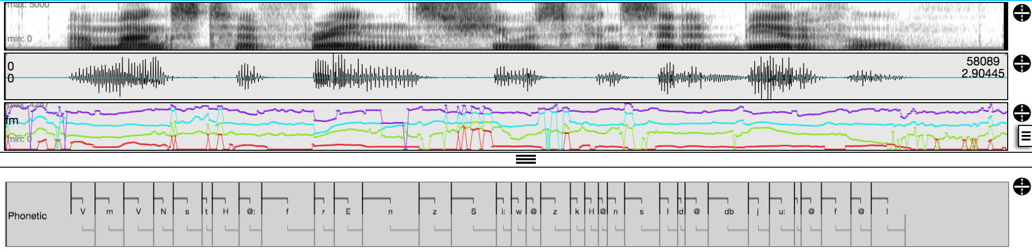
Figure 9.10: Screenshot of signal and level canvases displays of the EMU-webApp after the changes made in the above R code snippets.

9.3.3 Advanced configurations made by editing the _DBconfig.json

Although the above configuration options cover the most common use cases, the EMU-webApp offers multiple other configuration options that are currently not configurable via functions provided by emuR. These advanced configuration options can currently only be achieved by manually editing the _DBconfig.json file using a text editor. As even the colors used in the EMU-webApp and every keyboard shortcut can be reconfigured, here we will focus on the more common advanced configuration options. A full list of the available configuration fields of the EMUwebAppConfig section of the _DBconfig.json including their meaning, can be found in Appendix 15.1.1.

Overlaying signal canvases

To save space it can be beneficial to overlay one or more signal tracks onto other signal canvases. This can be achieved by manually editing the assign array of the EMUwebAppConfig:perspectives[persp_idx]:signalCanvases field in the _DBconfig.json. The Listing below shows an example configuration that overlays the fm track on the oscillogram where the OSCI string can be replaced by any other entry in the EMUwebAppConfig:perspectives[persp_idx]:signalCanvases:order array. Figure 9.11 displays a screenshot of such an overlay.

...
"assign": [{
    "signalCanvasName": "OSCI",
    "ssffTrackName": "fm"
}],
...

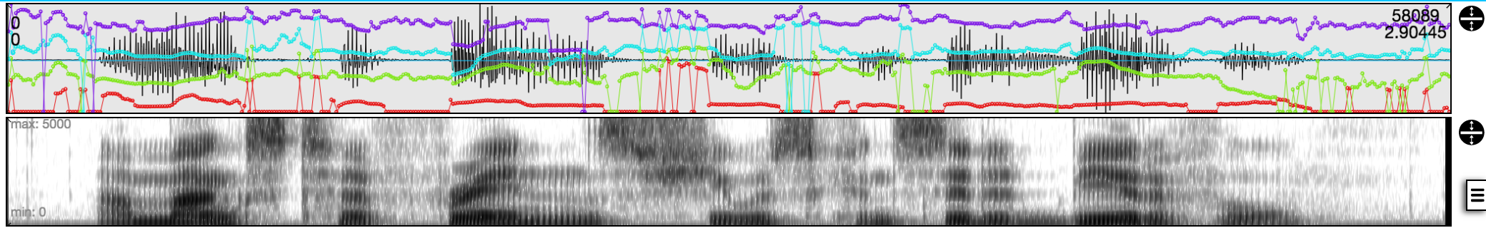
Figure 9.11: Screenshot of signal canvases display of the EMU-webApp after the changes made in the R code snippets above.

Frequency-aligned formant contours spectrogram overlay

The current mechanism for laying frequency-aligned formant contours over the spectrogram is to give the formant track the predefined name FORMANTS. If the formant track is called FORMANTS and it is assigned to be laid over the spectrogram (see Listing below) the EMU-webApp will frequency-align the contours to the current minimum and maximum spectrogram frequencies (see Figure 9.12).

...
"assign": [{
    "signalCanvasName": "SPEC",
    "ssffTrackName": "FORMANTS"
}],
...

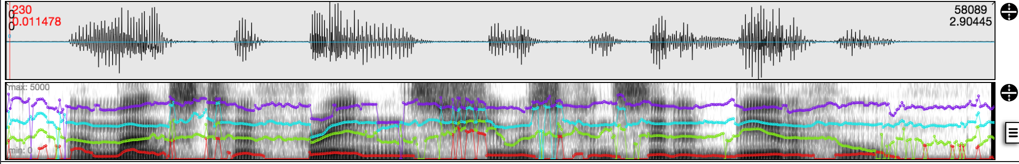
Figure 9.12: Screenshot of signal canvases area of the EMU-webApp displaying formant contours that are overlaid on the spectrogram and frequency-aligned.

Correcting formants

The above configuration of the frequency-aligned formant contours will automatically allow the FORMANTS track to be manually corrected. Formants can be corrected by hitting the appropriate number key (1 = first formant, 2 = second formant, …). Similar to boundaries and events, the mouse cursor will automatically be tracked in the SPEC canvas and the nearest formant value preselected. Holding down the SHIFT key moves the current formant value to the mouse position, hence allowing the contour to be redrawn and corrected.

9.3.4 2D canvas

The EMU-webApp has an additional canvas which can be configured to display two-dimensional data. Figure 9.13 shows a screenshot of the 2D canvas, which is placed in the bottom right hand corner of the level canvas area of the web application. The screenshot shows data representing EMA sensor positions on the mid sagittal plane. The Listing below shows how the 2D canvas can be configured. Essentially, every drawn dot is configured by assigning a column in an SSFF track that specifies the X values and an additional column that specifies the Y values.

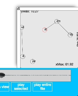
Figure 9.13: Screenshot of 2D canvas of the EMU-webApp displaying two-dimensional EMA data.

...
"twoDimCanvases": {
    "order": ["DOTS"],
    "twoDimDrawingDefinitions": [{
        "name": "DOTS",
        "dots": [{
            "name": "tt",
            "xSsffTrack": "tt_posy",
            "xContourNr": 0,
            "ySsffTrack": "tt_posz",
            "yContourNr": 0,
            "color": "rgb(255,0,0)"
        },
...
    "connectLines": [{
        "fromDot": "tt",
        "toDot": "tm",
            "color": "rgb(0,0,0)"
    },
...

EPG

The 2D canvas of the EMU-webApp can also be configured to display EPG data as displayed in Figure 9.14. The SSFF file containing the EPG data has to be formated in a specific way. The format is a set of eight bytes per point in time, where each byte represents a row of electrodes on the artificial palate. Each binary bit value per byte indicates whether one of the eight sensors is activated or not (i.e., tongue contact was measured). If data in this format and an SSFF track with the predefined name EPG referencing the SSFF files are present, the 2D canvas can be configured to display this data by adding the EPG to the twoDimCanvases:order array as shown in Listing below.

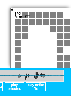
Figure 9.14: Screenshot of 2D canvas of the EMU-webApp displaying EPG palate traces.

"twoDimCanvases": {
    "order": ["EPG"]
}

EMA gestural landmark recognition

The EMU-webApp can also be configured to semi-automatically detect gestural landmarks of EMA contours. The functions implemented in the EMU-webApp are based on various Matlab scripts by Phil Hoole. For a description of which gestural landmarks are detected and how these are detected, see Bombien (2011) page 61 ff.

Compared to the above configurations, configuring the EMU-webApp to semi-automatically detect gestural landmarks of EMA contours is done as part of the level definition’s configuration entries of the _DBconfig.json. The Listing below shows the anagestConfig entry, which configures the tongueTipGestures event level for this purpose. Within the web application this level has to be preselected by the user and a region containing a gesture in the SSFF track selected (left click and drag). Hitting the ENTER/RETURN key then executes the semi-automatic gestural landmark recognition functions. If multiple candidates are recognized for certain landmarks, the user will be prompted to select the appropriate landmark.

...
"levelDefinitions": [{
  {
    "name": "tongueTipGestures",
    "type": "EVENT",
    "attributeDefinitions": [{
        "name": "tongueTipGestures",
        "type": "STRING"
    }],
    "anagestConfig": {
        "verticalPosSsffTrackName": "tt_posz",
        "velocitySsffTrackName": "t_tipTV",
        "autoLinkLevelName": "ORT",
        "multiplicationFactor": 1,
        "threshold": 0.2,
        "gestureOnOffsetLabels": ["gon", "goff"],
        "maxVelocityOnOffsetLabels": ["von", "voff"],
        "constrictionPlateauBeginEndLabels": ["pon", "poff"],
        "maxConstrictionLabel": "mon"
    }
...

The user will be prompted to select an annotation item of the level specified in anagestConfig:autoLinkLevelName once the gestural landmarks are recognized. The EMU-webApp then automatically links all gestural landmark events to that item.

9.4 Conclusion

This chapter provided an overview of the EMU-webApp by showing the main layout and configuration options and how its labeling mechanics work. To our knowledge, the EMU-webApp is the first client-side web-based annotation tool that is this feature rich. Being completely web-based not only allows it to be used within the context of the EMU-SDMS but also allows it to connect to any web server that implements the EMU-webApp-websocket-protocol (see Appendix 16 for details). This feature is currently being utilized, for example, by the IPS-EMUprot-nodeWSserver.js server side software package (see https://github.com/IPS-LMU/IPS-EMUprot-nodeWSserver), which allows emuDBs to be served to any number of clients for collaborative annotation efforts. Further, by using the URL Parameters (see Chapter 13 for details) the web application can also be used to display annotation data that is hosted on any web server.²⁰ Because of these features, we feel the EMU-webApp is a valuable contribution to the speech and spoken language software tool landscape.

---

16. Sections of this chapter have been published in (Winkelmann and Raess 2015) and some descriptions where taken from the EMU-webApp’s own manual.↩︎

17. This section is an updated version of the The level hierarchy section of the General Usage chapter that is part of the EMU-webApp own brief manual by Markus Jochim.↩︎

18. The term context menu is used in user interface design to refer to a pop-up menu or pop-up area that provides additional information for the current state (i.e., the current item).↩︎

19. If this side menu is not visible in your emuDB, make sure you have the EMUwebAppConfig: restrictions: showPerspectivesSidebar DBconfig entry set to true (see https://github.com/IPS-LMU/EMU-webApp/blob/master/app/testData/newFormat/ae/ae_DBconfig.json#L187 for an example)↩︎

20. See the BAS CLARIN Repository for a further example of an application using the EMU-webApp-websocket-protocol to display repository data in the EMU-webApp. See the BAS Web Services for an example of an application that creates links that utilize the URL parameters.↩︎