14 Use cases
To add to the tutorial of Chapter 3, this chapter will present a few short use cases extracted and updated from the emuR_intro vignette. These use cases are meant as practical guides to answering research questions and are to be viewed as generic template procedures that can be altered and applied to similar research questions. They are meant to give practical examples of what it is like working with the EMU-SDMS to answer research questions common in speech and spoken language research. Every use case will start off by asking a question about the ae demo database and will continue by walking through the process of answering this question by using the mechanics the emuR package provides. The four questions this chapter will address are:
- Section 14.1: What is the average length of all n phonetic segments in the ae
emuDB? - Section 14.2: What does the F1 and F2 distribution of all phonetic segments that contain the labels I, o:, u:, V or @ look like?
- Section 14.3: What words do the phonetic segments that carry the labels s, z, S or Z in the ae
emuDBoccur in and what is their phonetic context? - Section 14.4: Do the phonetic segments that carry the labels s, z, S or Z in the ae
emuDBdiffer with respect to their first spectral moment? \end{itemize}
The R code snippet below shows how the emuR demo data used in this chapter is created.
# load the package
library(emuR)

# create demo data in directory provided by the tempdir() function
create_emuRdemoData(dir = tempdir())

# get the path to emuDB called 'ae' that is part of the demo data
path2directory = file.path(tempdir(), "emuR_demoData", "ae_emuDB")

# load emuDB into current R session
ae = load_emuDB(path2directory)
14.1 What is the average length of all n phonetic segments in the ae emuDB?
The first thing that has to be done to address this fairly simple question is to query the database for all n segments. This can be achieved using the query() function as shown in the R code snippet below.
# query segments
sl = query(ae, query = "Phonetic == n")

# show first row of sl
head(sl, n = 1)
## # A tibble: 1 x 16
## labels start end db_uuid session bundle start_item_id end_item_id level
## <chr> <dbl> <dbl> <chr> <chr> <chr> <int> <int> <chr>
## 1 n 1032. 1196. 0fc618… 0000 msajc… 158 158 Phon…
## # … with 7 more variables: attribute <chr>, start_item_seq_idx <int>,
## # end_item_seq_idx <int>, type <chr>, sample_start <int>, sample_end <int>,
## # sample_rate <int>The second argument of the query() contains a string that represents an EQL statement. This fairly simple EQL statement consists of ==, which is the equality operator of the EQL, and on the right hand side of the operator the label n that we are looking for.
The query() function returns an object of the class emuRsegs that is a superclass of the well known data.frame. The various columns of this object should be fairly self-explanatory: labels displays the extracted labels, start and end are the start time and end times in milliseconds of each segment and so on. We can now use the information in this object to calculate the mean durations of these segments as shown in the R code snippet below.
# calculate durations
d = sl$end - sl$start

# calculate mean
mean(d)
## [1] 67.0583314.2 What does the F1 and F2 distribution of all phonetic segments that contain the labels I, o:, u:, V or @ look like?
Once again we will initially query the emuDB to retrieve the segments we are interested in as shown in the R code snippet below.
# query emuDB
sl = query(ae, query = "Phonetic == I|o:|u:|V|@")
Now that the necessary segment information has been extracted, the get\_trackdata() function can be used to calculate the formant values for these segments as displayed in the R code snippet below.
# get formant values for these segments
td = get_trackdata(ae,
                   sl,
                   onTheFlyFunctionName = "forest")
In this example, the get_trackdata() function uses a formant estimation function called forest() to calculate the formant values in real time. This signal processing function is part of the wrassp package, which is used by the emuR package to perform signal processing duties with the get_trackdata() command (see Chapter 8 for details).
If the resultType parameter is not set the call to get\_trackdata(), an object of the class tibble is returned. The class vector of the td object is displayed in the R code snippet below.
# show class vector of td
class(td)
## [1] "tbl_df" "tbl" "data.frame"# show td
td## # A tibble: 641 x 24
## sl_rowIdx labels start end db_uuid session bundle start_item_id end_item_id
## <int> <chr> <dbl> <dbl> <chr> <chr> <chr> <int> <int>
## 1 1 V 187. 257. 0fc618… 0000 msajc… 147 147
## 2 1 V 187. 257. 0fc618… 0000 msajc… 147 147
## 3 1 V 187. 257. 0fc618… 0000 msajc… 147 147
## 4 1 V 187. 257. 0fc618… 0000 msajc… 147 147
## 5 1 V 187. 257. 0fc618… 0000 msajc… 147 147
## 6 1 V 187. 257. 0fc618… 0000 msajc… 147 147
## 7 1 V 187. 257. 0fc618… 0000 msajc… 147 147
## 8 1 V 187. 257. 0fc618… 0000 msajc… 147 147
## 9 1 V 187. 257. 0fc618… 0000 msajc… 147 147
## 10 1 V 187. 257. 0fc618… 0000 msajc… 147 147
## # … with 631 more rows, and 15 more variables: level <chr>, attribute <chr>,
## # start_item_seq_idx <int>, end_item_seq_idx <int>, type <chr>,
## # sample_start <int>, sample_end <int>, sample_rate <int>, times_orig <dbl>,
## # times_rel <dbl>, times_norm <dbl>, T1 <int>, T2 <int>, T3 <int>, T4 <int>As the tibble class is a superclass to the common data.frame class, packages like ggplot2 can be used to visualize our F1 and F2 distribution as shown in the R code snippet below (see Figure 14.1 for the resulting plot).
# load package
library(ggplot2)

# scatter plot of F1 and F2 values using ggplot
ggplot(td, aes(x=T2, y=T1, label=td$labels)) +
  geom_text(aes(colour=factor(labels))) +
  scale_y_reverse() + scale_x_reverse() +
  labs(x = "F2(Hz)", y = "F1(Hz)") +
  guides(colour=FALSE)
## Warning: Use of `td$labels` is discouraged. Use `labels` instead.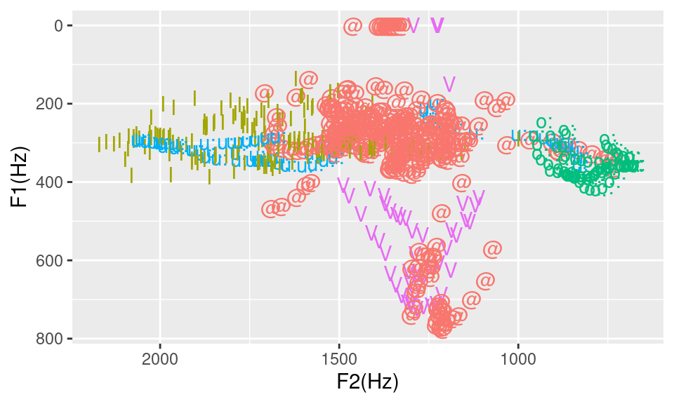
Figure 14.1: F1 by F2 distribution for I, o:, u:, V and *.
14.3 What words do the phonetic segments that carry the labels s, z, S or Z in the ae emuDB occur in and what is their phonetic context?
As with the previous use cases, the initial step is to query the database to extract the relevant segments as shown in the R code snippet below.
# query segments
sibil = query(ae, "Phonetic==s|z|S|Z")

# show sibil
sibil
## # A tibble: 32 x 16
## labels start end db_uuid session bundle start_item_id end_item_id level
## <chr> <dbl> <dbl> <chr> <chr> <chr> <int> <int> <chr>
## 1 s 483. 567. 0fc618… 0000 msajc… 151 151 Phon…
## 2 z 1196. 1289. 0fc618… 0000 msajc… 159 159 Phon…
## 3 S 1289. 1420. 0fc618… 0000 msajc… 160 160 Phon…
## 4 z 1548. 1634. 0fc618… 0000 msajc… 164 164 Phon…
## 5 s 1791. 1893. 0fc618… 0000 msajc… 169 169 Phon…
## 6 z 476. 572. 0fc618… 0000 msajc… 155 155 Phon…
## 7 z 2078. 2169. 0fc618… 0000 msajc… 178 178 Phon…
## 8 s 2228. 2319. 0fc618… 0000 msajc… 180 180 Phon…
## 9 s 2528. 2754. 0fc618… 0000 msajc… 185 185 Phon…
## 10 S 427. 546. 0fc618… 0000 msajc… 153 153 Phon…
## # … with 22 more rows, and 7 more variables: attribute <chr>,
## # start_item_seq_idx <int>, end_item_seq_idx <int>, type <chr>,
## # sample_start <int>, sample_end <int>, sample_rate <int>The requery_hier() function can now be used to perform a hierarchical requery using the set resulting from the initial query. This requery follows the hierarchical links of the annotations in the database to find the linked annotation items on a different level. The R code snippet below shows how this can achieved.
# perform requery
words = requery_hier(ae, sibil, level = "Word")

# show words
words
## # A tibble: 32 x 16
## labels start end db_uuid session bundle start_item_id end_item_id level
## <chr> <dbl> <dbl> <chr> <chr> <chr> <int> <int> <chr>
## 1 C 187. 674. 0fc618… 0000 msajc… 2 2 Word
## 2 C 740. 1289. 0fc618… 0000 msajc… 30 30 Word
## 3 F 1289. 1463. 0fc618… 0000 msajc… 43 43 Word
## 4 F 1463. 1634. 0fc618… 0000 msajc… 52 52 Word
## 5 C 1634. 2150. 0fc618… 0000 msajc… 61 61 Word
## 6 F 412. 572. 0fc618… 0000 msajc… 14 14 Word
## 7 C 1958. 2754. 0fc618… 0000 msajc… 80 80 Word
## 8 C 1958. 2754. 0fc618… 0000 msajc… 80 80 Word
## 9 C 1958. 2754. 0fc618… 0000 msajc… 80 80 Word
## 10 C 380. 745. 0fc618… 0000 msajc… 13 13 Word
## # … with 22 more rows, and 7 more variables: attribute <chr>,
## # start_item_seq_idx <int>, end_item_seq_idx <int>, type <chr>,
## # sample_start <int>, sample_end <int>, sample_rate <int>As seen in the above R code snippet, the result is not quite what one would expect as it does not contain the orthographic word transcriptions but a classification of the words into content words (C) and function words (F). Calling the summary() function on the emuDBhandle object ae would show that the Words level has multiple attribute definitions indicating that each annotation item in the Words level has multiple parallel labels defined for it. The R code snippet below shows an additional requery that queries the Text attribute definition instead.
# perform requery
words = requery_hier(ae, sibil, level = "Text")

# show words
words
## # A tibble: 32 x 16
## labels start end db_uuid session bundle start_item_id end_item_id level
## <chr> <dbl> <dbl> <chr> <chr> <chr> <int> <int> <chr>
## 1 among… 187. 674. 0fc618… 0000 msajc… 2 2 Word
## 2 frien… 740. 1289. 0fc618… 0000 msajc… 30 30 Word
## 3 she 1289. 1463. 0fc618… 0000 msajc… 43 43 Word
## 4 was 1463. 1634. 0fc618… 0000 msajc… 52 52 Word
## 5 consi… 1634. 2150. 0fc618… 0000 msajc… 61 61 Word
## 6 is 412. 572. 0fc618… 0000 msajc… 14 14 Word
## 7 resis… 1958. 2754. 0fc618… 0000 msajc… 80 80 Word
## 8 resis… 1958. 2754. 0fc618… 0000 msajc… 80 80 Word
## 9 resis… 1958. 2754. 0fc618… 0000 msajc… 80 80 Word
## 10 chill 380. 745. 0fc618… 0000 msajc… 13 13 Word
## # … with 22 more rows, and 7 more variables: attribute <chr>,
## # start_item_seq_idx <int>, end_item_seq_idx <int>, type <chr>,
## # sample_start <int>, sample_end <int>, sample_rate <int>As seen in the above R code snippet, the first segment in sibil occurred in the word amongst, which starts at 187.475 ms and ends at 674.225 ms. It is worth noting that this two-step querying procedure (query() followed by requery_hier()) can also be completed in a single hierarchical query using the dominance operator (^).
As we have answered the first part of the question, the R code snippet below will extract the context to the left of the extracted sibilants by using the requery_seq() function.
# get left context by off setting the
# annotation items in sibil one unit to the left
leftContext = requery_seq(ae, sibil, offset = -1)

# show leftContext
leftContext
## # A tibble: 32 x 16
## labels start end db_uuid session bundle start_item_id end_item_id level
## <chr> <dbl> <dbl> <chr> <chr> <chr> <int> <int> <chr>
## 1 N 427. 483. 0fc618… 0000 msajc… 150 150 Phon…
## 2 n 1032. 1196. 0fc618… 0000 msajc… 158 158 Phon…
## 3 z 1196. 1289. 0fc618… 0000 msajc… 159 159 Phon…
## 4 @ 1506. 1548. 0fc618… 0000 msajc… 163 163 Phon…
## 5 n 1741. 1791. 0fc618… 0000 msajc… 168 168 Phon…
## 6 I 412. 476. 0fc618… 0000 msajc… 154 154 Phon…
## 7 @ 2022. 2078. 0fc618… 0000 msajc… 177 177 Phon…
## 8 I 2169. 2228. 0fc618… 0000 msajc… 179 179 Phon…
## 9 n 2431. 2528. 0fc618… 0000 msajc… 184 184 Phon…
## 10 t 380. 427. 0fc618… 0000 msajc… 152 152 Phon…
## # … with 22 more rows, and 7 more variables: attribute <chr>,
## # start_item_seq_idx <int>, end_item_seq_idx <int>, type <chr>,
## # sample_start <int>, sample_end <int>, sample_rate <int>The R code snippet below attempts to extract the right context in the same manner as above R code snippet, but in this case we encounter a problem.
# get right context by off-setting the
# annotation items in sibil one unit to the right
rightContext = requery_seq(ae, sibil, offset = 1)
## Error in requery_seq(ae, sibil, offset = 1): 4 of the requested sequence(s) is/are out of boundaries.
## Set parameter 'ignoreOutOfBounds=TRUE' to get residual result segments that lie within the bounds.As can be seen by the error message in the above R code snippet, four of the sibilants occur at the very end of the recording and therefore have no phonetic post-context. The remaining post-contexts can be retrieved by setting the ignoreOutOfBounds argument to TRUE as displayed in the R code snippet below.
rightContext = requery_seq(ae, sibil,
                           offset = 1,
                           ignoreOutOfBounds = TRUE)
## Warning in requery_seq(ae, sibil, offset = 1, ignoreOutOfBounds = TRUE): Found
## missing items in resulting segment list! Replacing missing rows with NA values.# show rightContext
rightContext## # A tibble: 32 x 16
## labels start end db_uuid session bundle start_item_id end_item_id level
## <chr> <dbl> <dbl> <chr> <chr> <chr> <int> <int> <chr>
## 1 t 567. 597. 0fc618… 0000 msajc… 152 152 Phon…
## 2 S 1289. 1420. 0fc618… 0000 msajc… 160 160 Phon…
## 3 i: 1420. 1463. 0fc618… 0000 msajc… 161 161 Phon…
## 4 k 1634. 1676. 0fc618… 0000 msajc… 165 165 Phon…
## 5 I 1893. 1945. 0fc618… 0000 msajc… 170 170 Phon…
## 6 f 572. 674. 0fc618… 0000 msajc… 156 156 Phon…
## 7 I 2169. 2228. 0fc618… 0000 msajc… 179 179 Phon…
## 8 t 2319. 2345. 0fc618… 0000 msajc… 181 181 Phon…
## 9 <NA> NA NA <NA> <NA> <NA> NA NA <NA>
## 10 I 546. 615. 0fc618… 0000 msajc… 154 154 Phon…
## # … with 22 more rows, and 7 more variables: attribute <chr>,
## # start_item_seq_idx <dbl>, end_item_seq_idx <dbl>, type <chr>,
## # sample_start <int>, sample_end <int>, sample_rate <int>However, the resulting rightContext contains rows that only contain NA values. This indicates that no values where found for the corresponding row in the sibil segment list.
14.4 Do the phonetic segments labeled s, z, S or Z in the ae emuDB differ with respect to their first spectral moment?\footnote{The original version of this use case was written by Florian Schiel as part of the emuR_intro vignette that is part of the emuR package.
14.4.1 NOTE: See 21 for more up to date methods of performing spectral analysis
Once again, the segments of interest are queried first. The R code snippet below shows how this can be achieved, this time using the new regular expression operand of the EQL (see Chapter 6 for details).
sibil = query(ae,"Phonetic =~ '[szSZ]'")## Warning in query_labels(emuDBhandle, levelName = lvlName, intermResTableSuffix = intermResTableSuffix, : =~ now requires ^ if you wish to match the
## first character in a sequence i.e. 'a.*' now also matches
## 'weakness' as it contains the sequence. '^a.*'
## matches sequences that start with 'a.*'
## e.g. the word 'amongst'.The R code snippet below shows how the get_trackdata() function can be used to calculate the Discrete Fourier Transform values for the extracted segments.
dftTd = get_trackdata(ae,
                      seglist = sibil,
                      onTheFlyFunctionName = 'dftSpectrum',
                      resultType = "trackdata")
As the resultType parameter was not explicitly set, an object of the class trackdata is returned. This object, just like an object of the class emuRtrackdata, contains the extracted trackdata information. Compared to the emuRtrackdata class, however, the object is not “flat” and in the form of a data.table or data.frame but has a more nested structure (see ?trackdata for more details).
Since we want to analyze sibilant spectral data we will now reduce the spectral range of the data to 1000 - 10000 Hz. This is due to the fact that there is a lot of unwanted noise in the lower bands that is irrelevant for the problem at hand and can even skew the end results. To achieve this we can use a property of a trackdata object that also carries the class spectral, which means that it is indexed using frequencies. The R code snippet below shows how to use this feature to extract the relevant spectral frequencies of the trackdata object.
dftTdRelFreq = dftTd[, 1000:10000]The R code snippet below shows how the fapply() function can be used to apply the moments() function to all elements of dftTdRelFreq.
dftTdRelFreqMom = fapply(dftTdRelFreq, moments, minval = T)The resulting dftTdRelFreqMom object is once again a trackdata object of the same length as the dftTdRelFreq trackdata object. It contains the first four spectral moments as shown in the R code snippet below.
# show first row of data belonging
# to first element of dftTdRelFreqMom
dftTdRelFreqMom[1]$data[1,]
## [1] 5.335375e+03 6.469573e+06 6.097490e-02 -1.103308e+00The information stored in the dftTdRelFreqMom and sibil objects can now be used to plot a time-normalized version of the first spectral moment trajectories, color coded by sibilant class, using emuR’s dplot() function. The R code snippet below shows the R code that produces Figure 14.2.
dplot(dftTdRelFreqMom[, 1],
      sibil$labels,
      normalise = TRUE,
      xlab = "Normalized Time [%]",
      ylab = "1st spectral moment [Hz]")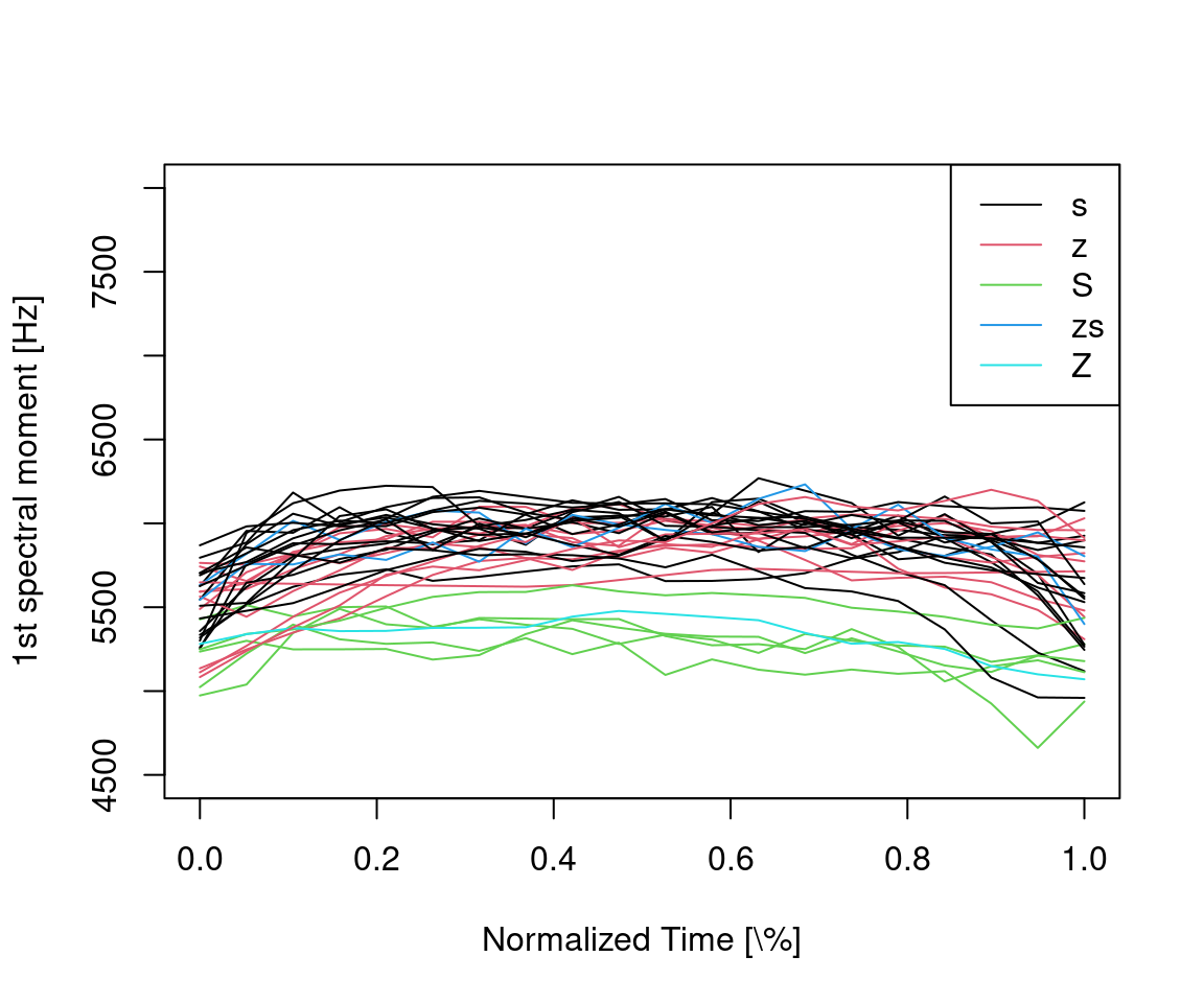
Figure 14.2: Time-normalized first spectral moment trajectories color coded by sibilant class.
As one might expect, the first spectral moment (the center of gravity) is significantly lower for postalveolar S and Z (green and blue lines) than for alveolar s and z (black and red lines).
The R code snippet below shows how to create an alternative plot (see Figure 14.3) that averages the trajectories into ensemble averages per sibilant class by setting the average parameter of dplot() to TRUE.
dplot(dftTdRelFreqMom[,1],
      sibil$labels,
      normalise = TRUE,
      average = TRUE,
      xlab = "Normalized Time [%]",
      ylab = "1st spectral moment [Hz]")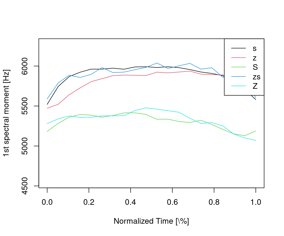
Figure 14.3: Time-normalized first spectral moment ensemble average trajectories per sibilant class.
As can be seen from the previous two plots (Figure 14.2 and 14.3), transitions to and from a sort of steady state around the temporal midpoint of the sibilants are clearly visible. To focus on this steady state part of the sibilant we will now extract those spectral moments that fall between the proportional timepoints 0.2 and 0.8 of each segment (i.e., the central 60%) using the dcut() function as is shown in the R code snippet below.
# cut out the middle 60% portion
dftTdRelFreqMomMid = dcut(dftTdRelFreqMom,
                          left.time = 0.2,
                          right.time = 0.8,
                          prop = T)
Finally, the R code snippet below shows how to calculate the averages of these trajectories using the trapply() function.
meanFirstMoments = trapply(dftTdRelFreqMomMid[,1],
                           fun = mean,
                           simplify = T)
As the resulting meanFirstMoments vector has the same length as the initial sibil segment list, we can now easily visualize these values in the form of a boxplot. The R code below shows the R code that produces Figure 14.4.
boxplot(meanFirstMoments ~ sibil$labels,
        xlab = "Sibilant class labels",
        ylab = "First spectral moment values [Hz]")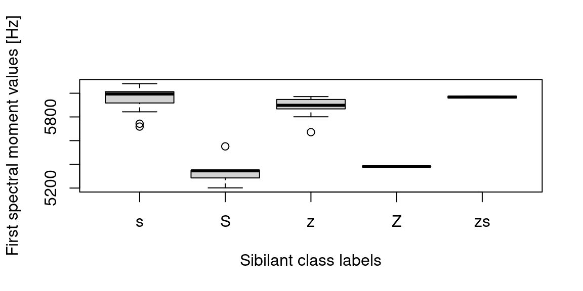
Figure 14.4: Boxplots of the first spectral moments grouped by their sibilant class.
As final remark, it is worth noting that using the emuRtrackdata resultType (not the trackdata resultType) of get_trackdata() function we could have performed a comparable analysis by utilizing packages such as dplyr for data.table or data.frame manipulation and lattice or ggplot2 for data visualisation.